Comb Filters

Comb Filters#

In this notebook, we’ll take a glimpse into how the digital audio signal processing tools we’ve developed so far can be useful in the design of digital audio effects, particularly artificial reverberation. Specifically we’ll look at two types of comb filters, which are the building blocks of more complex artificial reverberation systems.

Feedforward Comb Filter.#

Figure 1 depicts the block diagram of a feedforward comb filter, whose difference equation is given by:

\[ y[n] = x[n] + g x [n-N] \]

where N is the length of the delay (in samples), and g is a scalar gain. Given some sampling frequency, \(f_s\), the corresponding delay in seconds is \(N/f_s\).

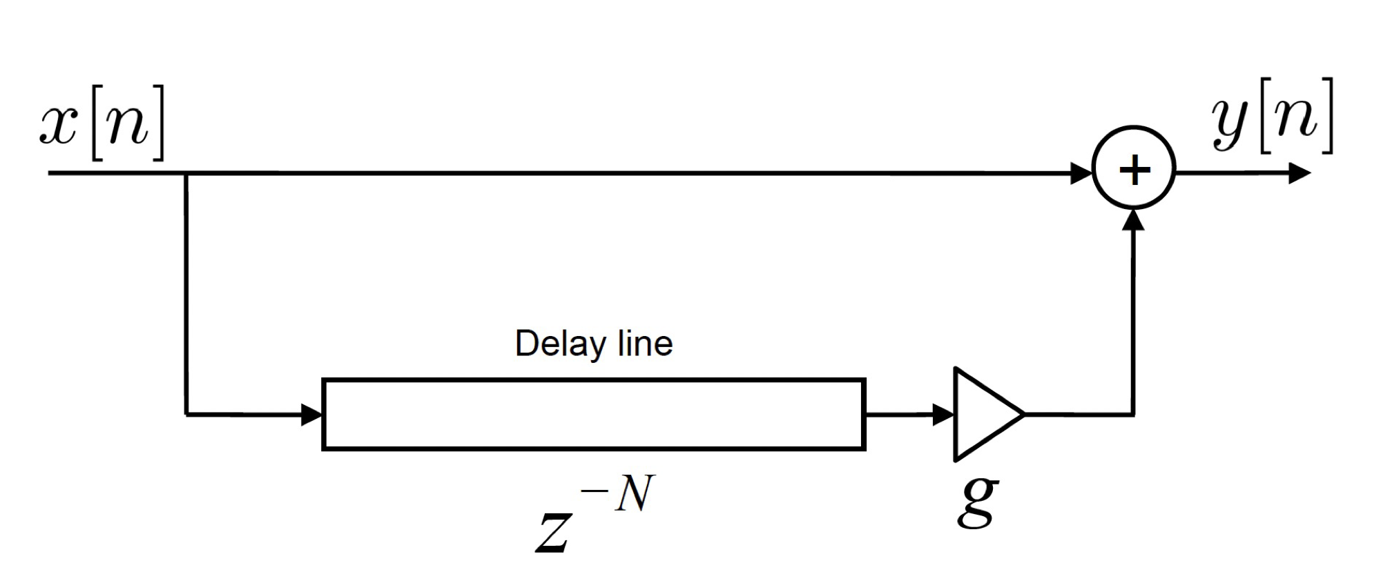
Fig. 1 - A feedforward comb filter.

Taking the Z-transform and re-arranging results in the transfer function of the feedforward comb filter:

\[ \begin{equation} H(z) = 1 + g z^{-N} \end{equation} \]

By comparing this expression to the transfer function for the general form of an \(N^{th}\) order LTI digital filter (from the previous notebook):

\[ \begin{align} H(z) &= \frac{b_0 + b_1z^{-1} + b_2z^{-2} + \dots + b_Nz^{-N}}{1 + a_1z^{-1} + a_2z^{-2} + \dots + a_Nz^{-N}} \end{align} \]

we can recognize that the feedforward filter will be Finite Impulse Response (FIR) filter as there is no denominator term (i.e., \(a_1 =a_2 =... a_N = 0\)). So for instance, if N = 2, the transfer function of the feedforward comb filter will be:

\[ \begin{equation} H(z) = 1 + g z^{-2} \end{equation} \]

where we deduce that \(b_0 = 1\), \(b_1=0\), and \(b_2=g\).

In the following interactive plot, we’ll observe how the impulse response of this filter (in time) and its corresponding Magnitude spectrum changes as we vary the delay length, \(N\) and the gain, \(g\). It should become very clear why we call this a “comb filter”! In order to build the filters, we’ll use the signal module within scipy python package and a sub-function called lfilter (https://docs.scipy.org/doc/scipy/reference/generated/scipy.signal.lfilter.html), where we can simply implement the filter by specifying the a and b coefficients.

# Building a basic feed forward comb filter line

# Initial parameters
fs = 5000                     # sampling frequency (Hz)
N_samples = 500               # total number of samples
n = np.arange(0,N_samples,1)  # This sets up a vector of the sample indices
x = np.zeros(N_samples);      # initial input
x[20] = 1                     # This makes x an impulse (the unit impulse occurs at sample index, n = 20)


fig, axes = plt.subplots(2,1, figsize=(8, 5)) 
fig.subplots_adjust(hspace=0.6)
line_input = axes[0].plot(n,x, label='input')
line_output, = axes[0].plot([],[],'--', label='output')
axes[0].set_xlabel('Number of samples')
axes[0].set_ylabel('Amplitude')
axes[0].set_ylim([0, 1])
axes[0].set_xlim([0, N_samples])
axes[0].legend()

line_mag, = axes[1].semilogx([],[])
axes[1].set_xlabel('Frequency (Hz)')
axes[1].set_ylabel('Magnitude (dB)')
axes[1].set_title('Magnitude resp of FeedFwd Comb Filter')
axes[1].set_xlim([10, fs//2])
axes[1].set_ylim([-30, 10])



# Starts the interactive plot.
def update(N = 10, g=0.1):
    
    # Create filter
    b = np.zeros(N+1)
    b[0] = 1    # first value of b
    b[-1] = g   # make the last value g (the final coefficient)
    a = 1       # this is the denominator
    
    # Run the filter to get the impulse response
    y_filt = signal.lfilter(b,a,x)  
    line_output.set_data(n, y_filt)
    axes[0].set_title('Delayed input by '+str(N)+' samples')
    
    # Get freq. response of the loop filter    
    [w,h] = signal.freqz(b,a, fs=fs,worN=fs)
    h_abs_dB = 10*np.log10(np.abs(h)**2) # express magnitude in dB
    line_mag.set_data(w,h_abs_dB)
    
    print('Listen to the impulse response')
    IPython.display.display(Audio(y_filt.T, rate=fs,normalize=True))
    
    fig.canvas.draw_idle()
    
    return 

N_s    = IntSlider(min=1, max=400, step=1, value=0, description='N')
g_s    = FloatSlider(min=0, max=0.99, step=0.01, value=1, description='g')

out = interactive_output(update, {'N': N_s, 'g': g_s} ); 
layout = widgets.VBox([N_s, g_s])
IPython.display.display(layout,out)

The sound of the feedforward comb filter#

At this point, we must be wondering what sonic impact the comb filter has on an input signal. The beauty of LTI system theory is that once we have the impulse response, all we need to do is do a convolution between the input signal and the impulse response to obtain the output. So let’s do exactly that in the following notebook and hear how the parameters \(N\) and \(g\) impact the sound of the input signal.

A few things to think about:

For what value of N does the effect transition from a reverberation-like sound to an echo-like sound?
What is the corresponding value of this transition point in milliseconds? (You will need the sampling frequency).
What does it tell us about our hearing from a psychoacoustic perspective?

# Read in the audio signal
x, fs = await read_wav_from_url(pan_sample) # read in the bass sample and get its sampling frequency (you can change 'pan_sample'  to 'bass_sample' or 'speech_sample')

# Convolution

N_samples = len(x)           # total number of samples
n = np.arange(0,N_samples,1) # This sets up a vector of the sample indices
tt = n/fs                    # vector in time (seconds)

# Input impulse
x_imp = np.zeros(N_samples); 
x_imp[0] = 1 # This makes x an impulse


fig, axes = plt.subplots(3,1, figsize=(8, 6)) 
fig.subplots_adjust(hspace=0.7)
line_input = axes[0].plot(tt,x, label='input')
axes[0].set_xlabel('Time (s)')
axes[0].set_ylabel('Amplitude')
axes[0].set_ylim([-1, 1])
axes[0].set_xlim([0, tt[-1]])
axes[0].set_title('Input Signal')

print("Listen to the input:")
IPython.display.display(Audio(x.T, rate=fs,normalize=True))


line_mag, = axes[1].semilogx([],[])
axes[1].set_xlabel('Frequency (Hz)')
axes[1].set_ylabel('Magnitude (dB)')
axes[1].set_title('Mag. Resp. of FeedFwd Comb Filter')
axes[1].set_xlim([10, fs//2])
axes[1].set_ylim([-30, 10])

line_output, = axes[2].plot([],[],'r', label='output')
axes[2].set_xlabel('Time (s)')
axes[2].set_ylabel('Filtered output')
axes[2].set_ylim([-1, 1])
axes[2].set_xlim([0, tt[-1]])



def update(N = 10, g=0.1):
    
    # Create filter:
    b = np.zeros(N+1)
    b[0] = 1    # first value of b
    b[-1] = g   # make the last value g (the final coefficient)
    a = 1       # this is the denominator

    # Get freq. response of the loop filter    
    [w,h] = signal.freqz(b,a, fs=fs,worN=fs)
    h_abs_dB = 10*np.log10(np.abs(h)**2) # express magnitude in dB
    line_mag.set_data(w,h_abs_dB)
    
    # # Run the filter 
    y_filt = signal.lfilter(b,a,x)  
    line_output.set_data(tt, y_filt)
    axes[2].set_title('Output Signal (Time delay  = '+str((N/fs)*1000)+' ms)')
    
    print("Listen to the output signal:")
    IPython.display.display(Audio(y_filt.T, rate=fs,normalize=True))
    IPython.display.clear_output(wait=True)

    fig.canvas.draw_idle()

print('Move the slider to see how the hyperparameters affect performance ')
interact(update, N = (0,4000,1), g=(0,0.99,0.01));
plt.show()

---------------------------------------------------------------------------
UnboundLocalError                         Traceback (most recent call last)
Cell In[12], line 2
      1 # Read in the audio signal
----> 2 x, fs = await read_wav_from_url(pan_sample) # read in the bass sample and get its sampling frequency (you can change 'pan_sample'  to 'bass_sample' or 'speech_sample')
      4 # Convolution
      6 N_samples = len(x)           # total number of samples

Cell In[8], line 29, in read_wav_from_url(url)
     28 async def read_wav_from_url(url):
---> 29     response = await pyfetch(url)
     30     wav_bytes = await response.bytes()  # get raw binary
     31     fs, data = wavfile.read(io.BytesIO(wav_bytes))

File ~/anaconda3/envs/acs_demos/lib/python3.8/site-packages/pyodide/http.py:232, in pyfetch(url, **kwargs)
    228 if IN_BROWSER:
    229     from js import fetch as _jsfetch, Object
    231 return FetchResponse(
--> 232     url, await _jsfetch(url, to_js(kwargs, dict_converter=Object.fromEntries))
    233 )

UnboundLocalError: local variable '_jsfetch' referenced before assignment

Feedback Comb Filter#

With the feedforward comb filter, we only consider a direct source and a single reflection. By alternatively doing the delay first and placing the gain in a feedback path, we can obtain a system that produces multiple reflections of progressively smaller amplitudes. This digital filter is referred to as a feedback comb filter and is depicted in Fig. 2.

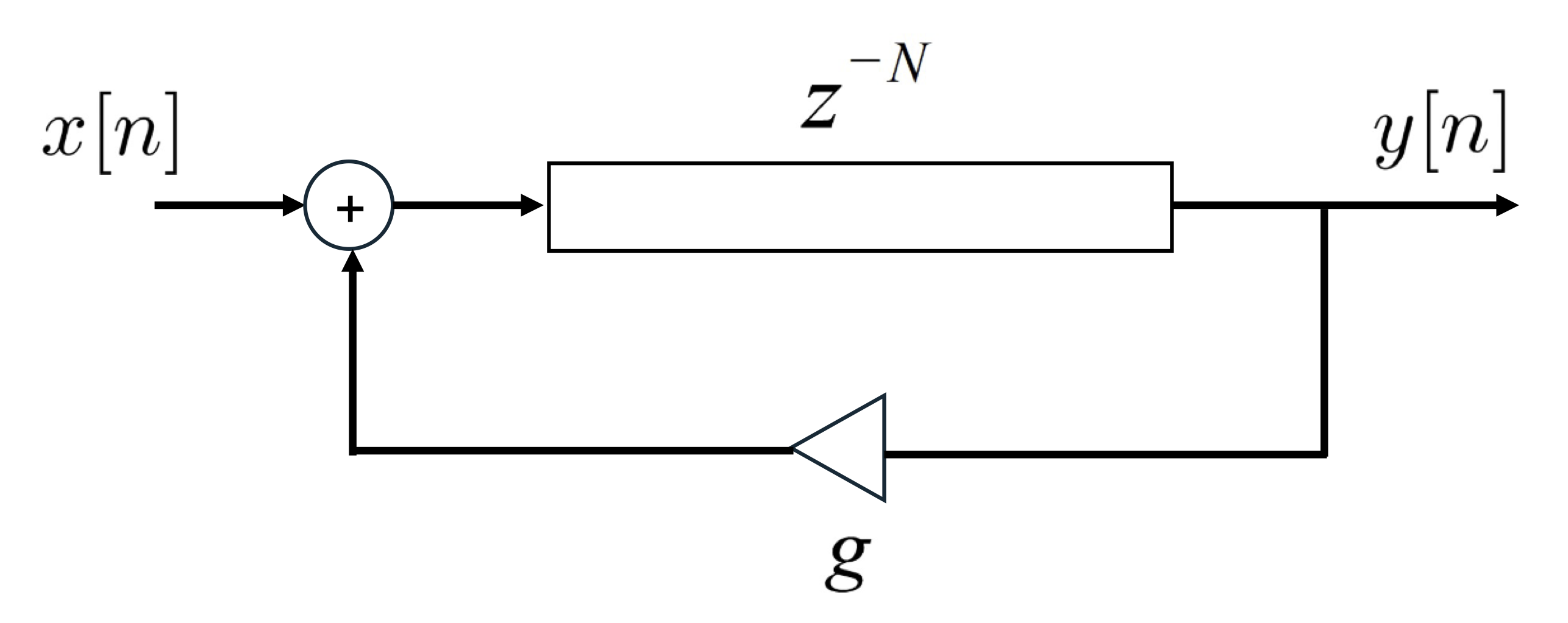
Fig. 2 - A feedback comb filter.

The transfer function of the feedback comb filter is now given by (you should be able to derive this by now!):

\[ \begin{equation} H(z) = \frac{z^{-N}}{1 - g z^{-N}} \end{equation} \]

We can that the feedback comb filter is an Infinite Impulse Response (IIR) filter as there are both numerator and denominator terms (in comparison to the feedforward comb filter, which was an FIR filter). The feedback comb filter has N zeros and N poles. The zeros all occur at \(z = 0\), whereas the poles are given by \(z = g^{1/N}\) (found by finding the value of z when the denominator of H(z) is zero). This corresponds to \(N\) poles equidistantly spaced around the unit circle, each with a magnitude of \(g^{1/N}\). The condition of stability of the feedback comb filter is given by \(|g| < 1\), as this ensures all the poles remain inside the unit circle.

Just as with the feedforward comb filter, in the following interactive plot, we’ll observe how the impulse response of the feedback filter (in time) and its corresponding Magnitude spectrum changes as we vary the delay length, \(N\) and the gain, \(g\). We will also observe the corresponding changes in the distribution of poles around the unit circle. We can also listen to the impulse response. How does the Magnitude spectrum compare with that of the feedforward comb filter?

# Initial parameters
fs = 5000                     # sampling frequency (Hz)
N_samples = 4000             # total number of samples
n = np.arange(0,N_samples,1)  # This sets up a vector of the sample indices
x = np.zeros(N_samples);      # initial input
x[20] = 1                    # This makes x an impulse

fig, axes = plt.subplot_mosaic([["top left", "top centre"],["top left", "bottom centre"]],figsize=(7.5,3))
plt.subplots_adjust(wspace=0.5,hspace=0.4)

# Create the unit circle
uc = patches.Circle((0,0), radius=1, fill=False, color='lightgray', ls='dashed')
axes["top left"].add_patch(uc)
 

# Plot the zeros and set marker properties    
t1, = axes["top left"].plot([], [], 'ko', ms=10)
plt.setp( t1, markersize=8.0, markeredgewidth=1.0,
          markeredgecolor='k', markerfacecolor='k')

# Plot the poles and set marker properties
t2, = axes["top left"].plot([], [], 'kx', ms=10)
plt.setp( t2, markersize=8.0, markeredgewidth=3.0,
          markeredgecolor='k', markerfacecolor='r')

axes["top left"].spines['left'].set_position('center')
axes["top left"].spines['bottom'].set_position('center')
axes["top left"].spines['right'].set_visible(False)
axes["top left"].spines['top'].set_visible(False)

axes["top left"].plot(1, 0, ">k", transform=axes["top left"].get_yaxis_transform(), clip_on=False)
axes["top left"].plot(0, 1, "^k", transform=axes["top left"].get_xaxis_transform(), clip_on=False)

# set the ticks
r = 1.1; 
axes["top left"].axis('scaled');
ticks_x = [-1, -0.5, 0.5, 1]; 
ticks_y = [-1, -0.5, 0.5, 1]; 
axes["top left"].set_xticks(ticks_x)
axes["top left"].set_yticks(ticks_y)
axes["top left"].text(1,0.1,'Real');
axes["top left"].text(0.1,1.1,'Imag');


line_input = axes["top centre"].plot(n,x, label='input')
line_output, = axes["top centre"].plot([],[],'--', label='output')
axes["top centre"].set_xlabel('Number of samples')
axes["top centre"].set_ylabel('Amplitude')
axes["top centre"].set_title('Imp. Resp. of Feedback Comb Filter')
axes["top centre"].set_ylim([0, 1])
axes["top centre"].set_xlim([0, N_samples])
axes["top centre"].legend()


# angles = np.unwrap(np.angle(h))
line_mag, = axes["bottom centre"].plot([], [], 'k')
axes["bottom centre"].set_xlabel('Frequency (Hz)')
axes["bottom centre"].set_ylabel('Magnitude (dB)')
axes["bottom centre"].set_title('Mag. Resp of Feedback Comb Filter')
axes["bottom centre"].set_xlim([10, fs//2])
axes["bottom centre"].set_ylim([-10, 25])

plt.tight_layout()
def update(N = 10, g=0.1):
    
    # Create filter
    b = np.zeros(N+1)
    a = np.zeros(N+1)
    b[-1] = 1   # make the last value g (the final coefficient)
    a[0] = 1    # this is the denominator first coefficient
    a[-1] = -g    # this is the denominator last coefficient
    
    # Run the filter to get the impulse response
    y_filt = signal.lfilter(b,a,x)  
    line_output.set_data(n, y_filt)
    #axes[0].set_title('Delayed input by '+str(N)+' samples')
    
    # Get freq. response of the loop filter    
    [w,h] = signal.freqz(b,a, fs=fs,worN=fs)
    h_abs_dB = 10*np.log10(np.abs(h)**2) # express magnitude in dB
    line_mag.set_data(w,h_abs_dB)
    
    # Get poles
    p = np.roots(a)
    t2.set_data(p.real, p.imag)
    t1.set_data(0, 0) # The zeros are all z = 0

    
    print('Listen to the impulse response')
    IPython.display.display(Audio(y_filt.T, rate=fs,normalize=True))

    fig.canvas.draw_idle()
        
    return 

N_s    = IntSlider(min=1, max=200, step=1, value=0, description='N')
g_s    = FloatSlider(min=0, max=1.2, step=0.01, value=0.9, description='g')

out = interactive_output(update, {'N': N_s, 'g': g_s} ); 
layout = widgets.VBox([N_s, g_s])
IPython.display.display(layout,out)

The sound of the feedback comb filter#

Just as we did with the feedforward comb filter, we can also listen to the result of applying a feedback comb filter to an audio signal for various values of \(N\) and \(g\). A few things to think about:

What are the differences in the sound of the feedback filter vs. the feedforward filter? Why?
What happens if the filter becomes unstable (i.e., when |g| > 1)? What is the resulting sound?
Does it sound like natural reverberation that you would perceive in a typical room? If not, how can it be improved?

# Convolution

x, fs = await read_wav_from_url(pan_sample) # read in the bass sample and get its sampling frequency (you can change 'pan_sample'  to 'bass_sample' or 'speech_sample')
N_samples = len(x)           # total number of samples
n = np.arange(0,N_samples,1) # This sets up a vector of the sample indices
tt = n/fs                    # vector in time (seconds)

# Input impulse
x_imp = np.zeros(N_samples); 
x_imp[0] = 1 # This makes x an impulse


fig, axes = plt.subplots(3,1, figsize=(8, 6)) 
fig.subplots_adjust(hspace=0.7)
line_input = axes[0].plot(tt,x, label='input')
axes[0].set_xlabel('Time (s)')
axes[0].set_ylabel('Amplitude')
axes[0].set_ylim([-1, 1])
axes[0].set_xlim([0, tt[-1]])
axes[0].set_title('Input Signal')

print("Listen to the input:")
IPython.display.display(Audio(x.T, rate=fs,normalize=True))


line_mag, = axes[1].semilogx([],[])
axes[1].set_xlabel('Frequency (Hz)')
axes[1].set_ylabel('Magnitude (dB)')
axes[1].set_title('Mag. Resp. of Feedback Comb Filter')
axes[1].set_xlim([10, fs//2])
axes[1].set_ylim([-20, 30])

line_output, = axes[2].plot([],[],'r', label='output')
axes[2].set_xlabel('Time (s)')
axes[2].set_ylabel('Filtered output')
axes[2].set_ylim([-1, 1])
axes[2].set_xlim([0, tt[-1]])



def update(N = 10, g=0.1):
    
    # Create filter:
    b = np.zeros(N+1)
    a = np.zeros(N+1)
    b[-1] = 1   # make the last value g (the final coefficient)
    a[0] = 1    # this is the denominator first coefficient
    a[-1] = -g    # this is the denominator last coefficient

    # Get freq. response of the loop filter    
    [w,h] = signal.freqz(b,a, fs=fs,worN=fs)
    h_abs_dB = 10*np.log10(np.abs(h)**2) # express magnitude in dB
    line_mag.set_data(w,h_abs_dB)
    
    # # Run the filter 
    y_filt = signal.lfilter(b,a,x)  
    line_output.set_data(tt, y_filt)
    axes[2].set_title('Output Signal (Time delay  = '+str((N/fs)*1000)+' ms)')
    
    print("Listen to the output signal:")
    IPython.display.display(Audio(y_filt.T, rate=fs,normalize=True))
    IPython.display.clear_output(wait=True)
    
    fig.canvas.draw_idle()


print('Move the slider to see how the hyperparameters affect performance ')
interact(update, N = (0,4000,1), g=(0,0.99,0.01));
plt.show()

Listen to the input:

Move the slider to see how the hyperparameters affect performance