import matplotlib
if not hasattr(matplotlib.RcParams, "_get"):
    matplotlib.RcParams._get = dict.get
Fourier transform#
Although the Fourier series has been quite fascinating, there was a shortcoming - it was only applicable for periodic signals and could only account for frequency components that were integer multiples of the fundamental. The Fourier transform on the other hand is more general in that it allows for analysis/synthesis of any type of signal and it can represent a continuous frequency spectrum. We’ll explore what all of this means in this notebook and derive the foundational tool for audio signal analysis - the Fourier transform.
The discrete frequency spectrum of the Fourier series#
Let’s start by considering the Fourier series of the periodic signal, \(f(t)\), illustrated in Fig. 1. This is a pulse-train type signal with period T_{o} and can be mathematically represented as
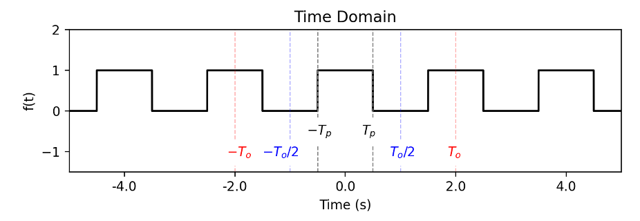
Fig. 1 - A pulse-train type signal with period To.
Let’s compute the coefficients of the Fourier series using the complex exponential form. Recall the formula to find the coefficients \(c_n\):
After working through is integral (your homework), we find that the coefficients \(c_n\) are given by (note that \(c_n\) has no imaginary parts, only real values):
Let’s plot the values of the \(c_n\) coefficients against angular frequency when \(T_p = 0.5\) and \(T_o = 2\). This is the amplitude spectrum of our signal, \(f(t)\) and is shown in Fig. 2. It tells us something about how the strength of the sinusoids is distributed across frequency. (In general, \(c_n\) is complex-valued, and in that case we tend to plot two things - the magnitude spectrum and the phase spectrum, i.e., the magnitude and phase of \(c_n\) against frequency).
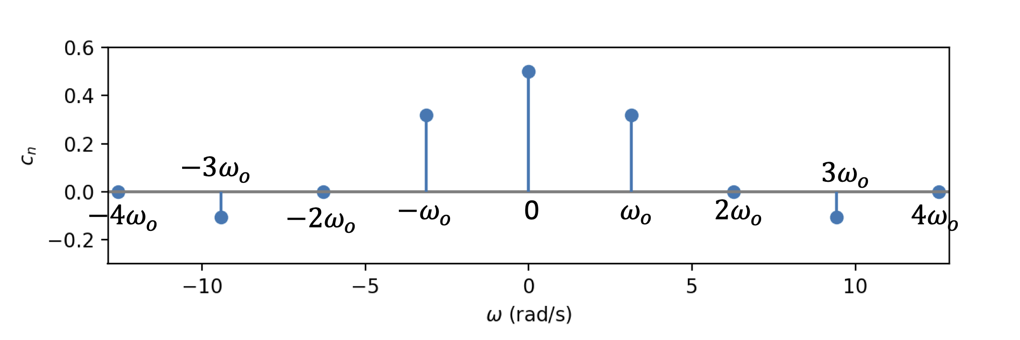
Fig. 2 - Amplitude spectrum of f(t).
There are a few important things to highlight in this plot:
The spectrum only consists of integer multiples of \(\omega_o\), i.e. \(n \omega_o\) for for \(n = 0, \pm 1, \pm 2, \dots \pm \infty\)
Hence we can think of the spectrum as discrete - only values at discrete frequencies, \(n \omega_o\) can be used to represent \(f(t)\). Frequencies in between these discrete values are undefined and cannot be used to represent \(f(t)\)
This is a direct consequence of the fact that we are dealing with periodic signals with a period \(T_o = 2 \pi /\omega_o\)
From the Fourier Series to the Fourier Transform (1)#
We know that signals we encounter on an everyday basis are not always periodic. For more complicated signals in comparison to the ones we’ve seen, there may not be a fundamental period that one can identify. We call such signals aperiodic. So how can we obtain the frequency content of aperiodic signals? Can we develop a similar framework to Fourier Series in order to treat aperiodic signals?
This is where the Fourier transform comes in to help us. We can think of the Fourier Transform as generalization of the Fourier Series that can also deal with aperiodic signals. It’s not always so intuitive, but we’ll use some interactive plots to hopefully clear this up.
Let’s start by making an aperiodic signal from a periodic one. We’ll use the same pulse-train type signal from above. In order to do this, we make the period infinite, i.e. we set \(T_{o} \rightarrow \infty\). In practical terms, what that means is that the period is much larger than the window of time for which we are observing the signal. Run the interactive plot below and increase \(T_o\) to see how we go from the periodic signal of the pulse-train to an aperiodic one, represented by a single pulse.
Tp = 0.5 # Pulse Width
To = 2

# The functions were taken from here (thanks!): https://stackoverflow.com/questions/29698213/rectangular-pulse-train-in-python
def rect(Tp):
    """ a function to return a centered rectangular pulse of width Tp """
    return lambda t: (-Tp <= t) & (t < Tp)

def pulse_train(t, at, shape):
    """create a train of pulses over t at times at and shape """
    return np.sum(shape(t - at[:,np.newaxis]), axis=0)

fig, axes = plt.subplots(figsize=(6, 2))

# Time domain plots
dt = 0.0001 # time spacing
t = np.arange(-5*To, 5*To, dt) # Range of times to plot
line, = axes.plot([], [], 'k')
vline = axes.axvline(To, color='red', linestyle='--', linewidth=0.8,alpha=0.3)  # Draw horizontal line at y=0
vline2 = axes.axvline(-To, color='red', linestyle='--', linewidth=0.8,alpha=0.3)  # Draw horizontal line at y=0
label1 = axes.text(To-0.2, -1.2, '$T_{o}$', color='red', ha='left', va='bottom', backgroundcolor='white')
label2 = axes.text(-To-0.2, -1.2, '$-T_{o}$', color='red', ha='left', va='bottom', backgroundcolor='white')

vline3 = axes.axvline(To/2, color='blue', linestyle='--', linewidth=0.8, alpha=0.3)  # Draw horizontal line at y=0
vline4 = axes.axvline(-(To/2), color='blue', linestyle='--', linewidth=0.8, alpha=0.3)  # Draw horizontal line at y=0
label3 = axes.text((To/2)-0.2, -1.2, '$T_{o}/2$', color='blue', ha='left', va='bottom', backgroundcolor='white')
label4 = axes.text(-(To/2)-0.5, -1.2, '$-T_{o}/2$', color='blue', ha='left', va='bottom', backgroundcolor='white')

vline5 = axes.axvline(Tp, color='grey', linestyle='--', linewidth=0.8)  # Draw horizontal line at y=0
vline6 = axes.axvline(-Tp, color='grey', linestyle='--', linewidth=0.8)  # Draw horizontal line at y=0

label5 = axes.text(Tp-0.2, -0.7, '$T_{p}$', color='black',  ha='left', va='bottom', backgroundcolor='white')
label6 = axes.text(-Tp-0.2, -0.7, '$-T_{p}$', color='black', ha='left', va='bottom', backgroundcolor='white')


axes.set_ylabel('f(t)', color='k')
axes.set_xlabel('Time (s)', color='k')
axes.xaxis.set_major_formatter(FormatStrFormatter('%.1f'))
axes.set_xlim([-5, 5])
axes.set_ylim([-1.5, 2])


def update(To = 2):

    # Time domain plots

    y = pulse_train(t=t,at=np.arange(-5*To, 5*To, To),shape=rect(Tp))
    fig.canvas.draw_idle()
    line.set_data(t, y)

    vline.set_xdata([To, To])
    vline2.set_xdata([-To, -To])
    label1.set_x(To-0.15)
    label2.set_x(-To-0.15)
    vline3.set_xdata([To/2, To/2])
    vline4.set_xdata([-To/2, -To/2])
    label3.set_x((To/2)-0.2)
    label4.set_x(-(To/2)-0.5)


print('See how the signal changes as we increase the period:')
interact(update, To = (2,20,0.1));
See how the signal changes as we increase the period:
From the Fourier Series to the Fourier Transform (2)#
Okay so we have set \(T_{o} \rightarrow \infty\). What consequences does this have on the math for computing the coefficients, \(c_n\) from the Fourier series analysis equation? Recall the formula for \(c_n\):
The first thing we can observe is that the limits of the integral will change. We can also multiply out by \(T_o\) to simplify things a bit:
Now recall that \(\omega_o = 2\pi/T_o\), which means that
That all feels really weird, but here is the key - in the Fourier Series, the spacing between the discrete frequencies is also \(\omega_o\) (shown in Fig. 3) and hence the spacing between these discrete frequencies decreases, i.e. it also tends to 0.
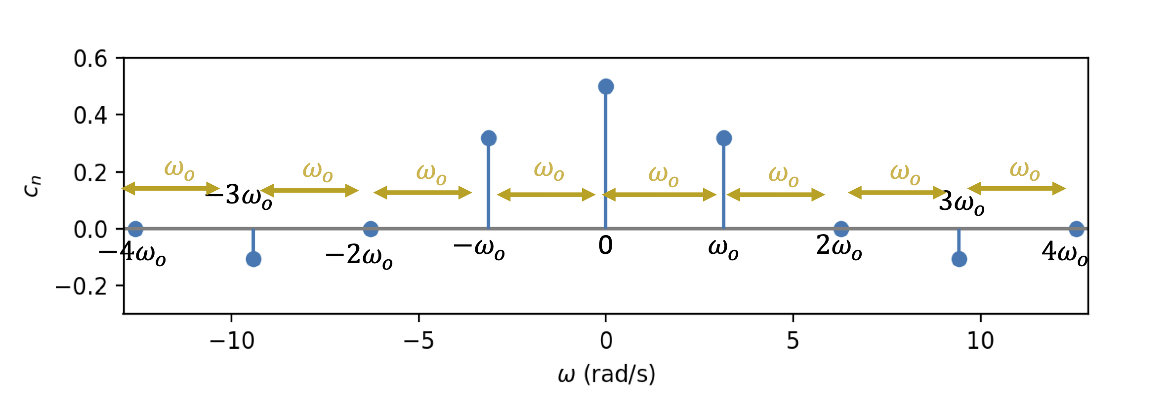
Fig. 2 - Amplitude spectrum of f(t) explicitly showing spacing between components.
Let’s visualize what we mean in the following interactive plot. Change \(T_o\) and see how things change in both the time and frequency domain.
Tp = 0.5 # Pulse Width

fig, axes = plt.subplots(2,1)
plt.subplots_adjust(hspace=0.7)

# Time domain plots

dt = 0.0001 # time spacing
t = np.arange(-5*To, 5*To, dt) # Range of times to plot
line, = axes[0].plot([], [], 'k')
vline = axes[0].axvline(To, color='red', linestyle='--', linewidth=0.8,alpha=0.3)  # Draw horizontal line at y=0
vline2 = axes[0].axvline(-To, color='red', linestyle='--', linewidth=0.8,alpha=0.3)  # Draw horizontal line at y=0
label1 = axes[0].text(To-0.2, -1.2, '$T_{o}$', color='red', ha='left', va='bottom', backgroundcolor='white')
label2 = axes[0].text(-To-0.2, -1.2, '$-T_{o}$', color='red', ha='left', va='bottom', backgroundcolor='white')

vline3 = axes[0].axvline(To/2, color='blue', linestyle='--', linewidth=0.8, alpha=0.3)  # Draw horizontal line at y=0
vline4 = axes[0].axvline(-(To/2), color='blue', linestyle='--', linewidth=0.8, alpha=0.3)  # Draw horizontal line at y=0
label3 = axes[0].text((To/2)-0.2, -1.2, '$T_{o}/2$', color='blue', ha='left', va='bottom', backgroundcolor='white')
label4 = axes[0].text(-(To/2)-0.5, -1.2, '$-T_{o}/2$', color='blue', ha='left', va='bottom', backgroundcolor='white')

vline5 = axes[0].axvline(Tp, color='grey', linestyle='--', linewidth=0.8)  # Draw horizontal line at y=0
vline6 = axes[0].axvline(-Tp, color='grey', linestyle='--', linewidth=0.8)  # Draw horizontal line at y=0

label5 = axes[0].text(Tp-0.2, -0.7, '$T_{p}$', color='black',  ha='left', va='bottom', backgroundcolor='white')
label6 = axes[0].text(-Tp-0.2, -0.7, '$-T_{p}$', color='black', ha='left', va='bottom', backgroundcolor='white')


axes[0].set_ylabel('f(t)', color='k')
axes[0].set_xlabel('Time (s)', color='k')
axes[0].xaxis.set_major_formatter(FormatStrFormatter('%.1f'))
axes[0].set_xlim([-5, 5])
axes[0].set_ylim([-1.5, 2])
axes[0].set_title('Time Domain', color='k')


# Freq domain plots

f_int = np.arange(-100, 101, 1) # Range of integer frequencies to plot
T_ak = np.zeros(len(f_int))

markers, = axes[1].plot([],[], ls="none", marker="o")
baseline = axes[1].axhline(0, color="grey")

verts=np.c_[f_int, np.zeros_like(f_int), f_int, T_ak].reshape(len(T_ak),2,2)
col = collections.LineCollection(verts)
axes[1].add_collection(col)


line_Freq, = axes[1].plot([], [], 'b')
axes[1].set_xlim([-2*4*np.pi, 2*4*np.pi])
axes[1].set_ylim([-0.5, 1.2])
axes[1].set_ylabel('$T_o  c_n$', color='k')
axes[1].set_xlabel('$\omega$ (rad/s)', color='k')
axes[1].set_title('Frequency Domain', color='k')

def update(To = 2):

    # Time domain plots

    y = pulse_train(t=t,at=np.arange(-5*To, 5*To, To),shape=rect(Tp))
    fig.canvas.draw_idle()
    line.set_data(t, y)

    vline.set_xdata([To, To])
    vline2.set_xdata([-To, -To])
    label1.set_x(To-0.15)
    label2.set_x(-To-0.15)
    vline3.set_xdata([To/2, To/2])
    vline4.set_xdata([-To/2, -To/2])
    label3.set_x((To/2)-0.2)
    label4.set_x(-(To/2)-0.5)


    # Frequency Domain plots
    wo = (2*np.pi)/To

    for n in range(len(f_int)):
        k = f_int[n]
        if k == 0:
            T_ak[n] = (2*Tp)
        else:
            T_ak[n] = (2*np.sin(k*wo*Tp))/(k*wo)

    markers.set_data(f_int*wo, T_ak)
    verts=np.c_[f_int*wo, np.zeros_like(f_int*wo), f_int*wo, T_ak].reshape(len(f_int*wo),2,2)
    col.set_segments(verts)


print('See how the signal changes as we increase the period:')
interact(update, To = (2,20,0.1));
See how the signal changes as we increase the period:
From the Fourier Series to the Fourier Transform (3)#
We essentially have gone from a discrete spectrum to a continuous one, i.e, as \(T_o \rightarrow \infty\), \(n \omega_o \rightarrow \omega\). This now means we can accommodate for any frequency! No longer are we constrained to integer multiples of \(\omega_o\). Returning to the math, what we end up with is
This integral is what we call the Fourier transform! Conventionally, we write it as follows
It’s still an audio analysis equation, i.e., it takes an input of the time-domain signal, \(f(t)\) and spits out a complex number, \(F(j\omega)\) for each value of \(\omega\), i.e., at all frequencies along a continuum (recall that \(\omega = 2 \pi f\), where \(f\) is the frequency in Hz). This allows us to quantify the magnitude and phase of our signal across frequency. Just as in the Fourier series, we can interpret this integral as computing a correlation between the signal \(f(t)\) and a complex exponential, but now at any frequency \(\omega\).
On a side note, it’s a matter of convention on how you will see it in literature. Here I’m writing the left-hand side as a function of \(j \omega\) to remind us that the values we obtain are complex-valued and as a function of frequency. Recall also that \(\omega = 2 \pi f\), where \(f\) is the frequency in Hz. Hence in some literature, you may find the left-hand side written as \(F(jf)\), \(F(f)\) or simply \(F(\omega)\).
We can also go the other way around and do synthesis if we have \(F(j\omega)\). This is what we call the inverse Fourier transform and is given by
An example#
Let’s go through an example to get a feel for how the Fourier transform works. Let’s consider a decaying exponential signat, \(f(t)\), which is defined as
To obtain the Fourier transform of this signal, we simply apply the Fourier transform analysis formula as and go through the integration:
We have now two domains in which we can fully analyze the signal - time time domain (a function of \(t\)) and the frequency domain, a function of \(\omega\). As we can observe, \(F(j\omega)\) is indeed a complex number. This means that we can obtain both the magnitude (absolute value of the complex number) and the phase (argument of the complex number) for any frequency, \(\omega\). Let’s plot this below and see how the magnitude and phase changes as we vary the parameter \(a\).
a = 0.5 # decay constant

fig, axes = plt.subplots(2,1)
plt.subplots_adjust(hspace=0.7)

# Time domain plots

dt = 0.001 # time spacing
t = np.arange(-5, 5, dt) # Range of times to plot
line, = axes[0].plot([], [], 'k')
axes[0].set_ylabel('f(t)', color='k')
axes[0].set_xlabel('Time (s)', color='k')
axes[0].xaxis.set_major_formatter(FormatStrFormatter('%.1f'))
axes[0].set_xlim([-5, 5])
axes[0].set_ylim([-0.5, 1.2])
axes[0].set_title('Time Domain', color='k')


# Freq domain plots

om_range = np.arange(-10, 10, 0.01) # Range of angular frequencies to plot
F_jw = np.zeros(len(om_range), dtype=complex) # Fourier Transform values

# markers, = axes[1].plot([],[], ls="none", marker="o")
# baseline = axes[1].axhline(0, color="grey")


line_Freq_mag, = axes[1].plot([], [])

axes[1].set_xlim([-2*np.pi, 2*np.pi])
axes[1].set_ylim([-0.7, 10])
axes[1].set_ylabel('$|F(j\omega)|$', color='b')
axes[1].set_xlabel('$\omega$ (rad/s)')
axes[1].set_title('Frequency Domain', color='k')


#make secondary y-axis for phase
ax2 = axes[1].twinx()
line_Freq_phase, = ax2.plot([], [],'orange')
ax2.set_ylabel('Phase of $F(j\omega)$', color='orange')
ax2.set_ylim([-np.pi, np.pi])


def update(a = 0.2):

    fig.canvas.draw_idle()

    # Time domain plots
    y = np.exp(-a*t)
    y[t<0] = 0

    line.set_data(t, y)

    # Frequency Domain plots
    F_jw = 1/(a + 1j*om_range)
    F_jw_mag = np.abs(F_jw)
    F_jw_phase = np.angle(F_jw)
    line_Freq_mag.set_data(om_range, F_jw_mag)
    line_Freq_phase.set_data(om_range, F_jw_phase)
    # line_Freq_mag.set_data(f_int*wo, T_ak)


print('See how the time domain and frequency domain characteristics of the signal changes as we vary the parameter, a:')
interact(update, a = (0.1,1,0.1));
See how the time domain and frequency domain characteristics of the signal changes as we vary the parameter, a:
Fourier Transform properties#
There are many interesting properties of the Fourier transform but I will not bore you with all of those details right now. Sometimes it can be more helpful to firstly work on problems to get more familiar with the Fourier transform and then look into these properties, where we may find greater appreciation for them. There is, however, one property that’s worth highlighting already and is perhaps already evident from the previous magnitude and phase plots. When a Fourier transform is taken of a real-valued signal in the time-domain, the magnitude and phase of the Fourier transform coefficients always have a particular relationship!
The magnitude is an even function, i.e. the values for \(\omega > 0\) are the same as those for \(\omega < 0\), i.e., \(|F(j\omega)| = |F(-j\omega)|\).
The phase is an odd function, i.e. the values for \(\omega > 0\) are the negative of those for \(\omega < 0\), i.e., \(\angle F(j\omega) = - \angle F(-j\omega)\).
Take some time to digest this by observing the previous plots again. It may not immediately appear relevant, but the bigger consequence of these relations is that we only need to know the values for half of the spectrum in order to have ALL the information related to the signal. For instance, if we wanted to synthesize any real-valued time-domain signal and all we know is half of the spectrum (positive or negative side); we can use these relations to obtain the missing halves, and subsequently use the inverse Fourier transform to obtain the real-valued time-domain signal. If these relations were not satisfied, the time-domain signal that you would synthesize would be complex-valued.