import matplotlib
if not hasattr(matplotlib.RcParams, "_get"):
    matplotlib.RcParams._get = dict.get
Time Frequency Analysis#
Towards the end of the previous chapter, we saw that doing frequency analysis on short time frames or segments within a long audio recording can reveal how the signal strength in various frequency components can change over time. We’ll formalize this concept a bit more and introduce the short-time Fourier transform (STFT) and the spectrogram.
Time-frequency representation#
Time-frequency representations of signals allow us to quantify the nature of signals in terms of its spectral (frequency) variations over time. As illustrated in Fig. 1, time-frequency analysis involves the conversion of our signal in terms of time and amplitude to a “grid-like” representation where one axis represents time frames (some time segment of the signal) and the other frequency (recall that the frequency bins are simply the discrete indices corresponding to each of the frequencies, \(k = 0, 1, 2, \dots N-1\)). At each of these time-frequency points, we can define some quantity which tells us something about the strength of the signal at those times and frequencies, e.g., a power spectral density.
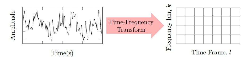
Fig. 1 - Transforming from the time-domain to a time-frequency domain
In this chapter, the time-frequency domain that will be used is the short-time Fourier transform (STFT), where the frequency scale is linear, meaning that there is a constant difference between adjacent frequency bins (i.e. each of the grid points in Fig. 1 is uniformly spaced in frequency). Other time-frequency transforms may however use non-linear frequency scales such as the [Mel scale](https://en.wikipedia.org/wiki/Mel_scale) or the equivalent [rectangular bandwidth (ERB)](https://en.wikipedia.org/wiki/Equivalent_rectangular_bandwidth).
Short time Fourier Transform (STFT)#
Fig. 2 depicts the processing steps to obtain the STFT representation starting from the discrete-time domain signal, \(x[n]\) in the upper-most plot. In the second step, \(x[n]\) is segmented into fixed-length overlapping frames each consisting of \(N\) samples. Each time frame is then multiplied by a window, \(w[n]\) as depicted in the second row of Fig. 2. Moving to the third row of Fig. 2, the \(l^{th}\) windowed time frame can be mathematically defined as
for \(n = [0, 1, . . . , N − 1]\), \(l = [0, 1, . . . , L − 1]\), where L is the total number of time frames, and R is the hop-size in samples. R directly defines the amount of overlap between frames, so for instance, if R = 256 and P = 512, then the amount of overlap is defined as 50%.
The final step of the STFT then involves taking a discrete Fourier transform (DFT) on each of these windowed time frames, \(\bar{x} [n, l]\), which yields complex-valued STFT coefficients:
where \(k = [0, 1, . . . , N − 1]\) is the frequency bin corresponding to the specific frequency (Hz), \(f = \frac{k f_s}{N}\), where \(f_s\) is the sampling frequency (Hz). With this, we now have the complex values \(X(k,l)\) that can be assembled as per the matrix/tile type representation as shown on the right-hand-side illustration of Fig. 1.
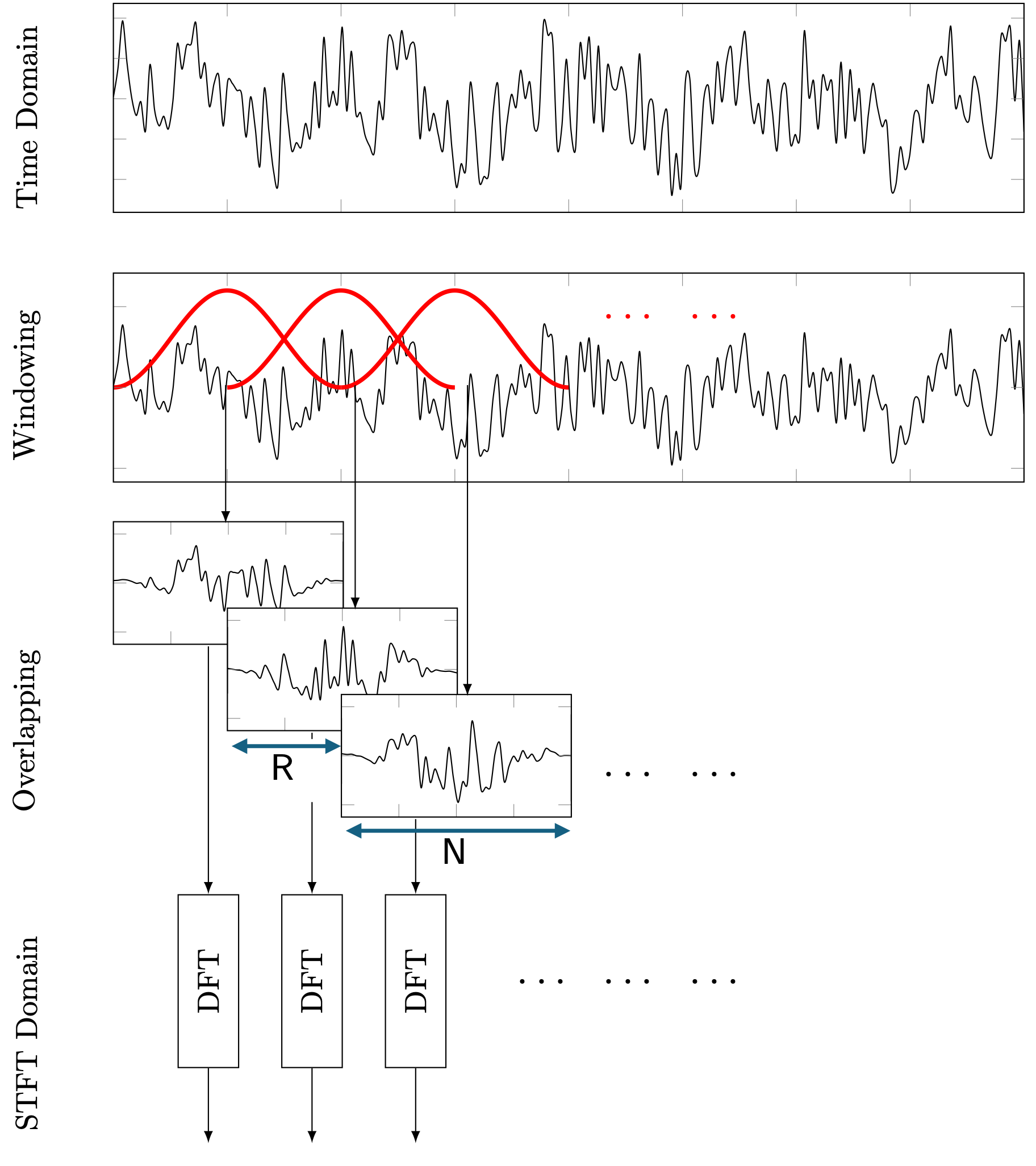
Fig. 2 - Short time Fourier Transform (STFT) process
Let’s begin by importing our audio signal. We’ll use the same vocal sample as before, but there’s also a recording of a Barred Antshrike that you can observe (simply change the variable ‘vocal’ to ‘birdcall’ in the code below).
# Import  signal
xx, fs = await read_wav_from_url(vocal)   # if you want to observe the bird call, change 'vocal' to 'birdcall' - we imported these URLs above.
t = np.arange(0,len(xx),1)*(1/fs) # time vector

IPython.display.display(Audio(xx.T, rate=fs))

fig, axes = plt.subplots(figsize=(6, 3))
axes.plot(t, xx)
axes.set_xlabel('Time (s)')
axes.set_ylabel('Amplitude')
plt.tight_layout()
plt.show()
/var/folders/ng/90xk1wjn2014rw8nb9bql2200000gp/T/ipykernel_32667/1889954770.py:2: WavFileWarning: Chunk (non-data) not understood, skipping it.
  fs, xx = wavfile.read('../audio/vocal_sample.wav')
Spectrograms and Time/Frequency Resolution#
Okay, now that we have imported our time domain signal and we know the sampling frequency of the signal, the next step is to compute the STFT of the signal. We in fact have built up all the tools required to code this up ourselves! We could alternatively use the scipy.signal.spectrogram function, but building our own functions gives us more insight and control into the analysis of the signals - we know what the equations are going into it.
After computing the STFT of the signal, the result can be plotted in what we call a Spectrogram, where the magnitude, magnitude-squared, or power spectral density of the DFT coefficients are displayed as a colourmap over time and frequency. We will also use the imshow function in Python, typically used for plotting images, to plot the spectrogram. Essentially we’ll store the data in a matrix and plot that matrix as an “image”.
One of the parameters we need to choose before computing the STFT however, is the length of the time frames, \(N\) (i.e. the number of samples over which we compute the DFT, see Fig. 2). Recalling our previous formula for the frequency, \(f = kf_{s}/N\), for \(k = [0, 1, . . . , N − 1]\), we can define the frequency resolution, i.e. the spacing between each freuqency bin as:
This equation tells us that we can essentially increase our frequency resolution by reducing the sampling frequency, \(f_s\) or by increasing the number of of samples in each time frame, \(N\). However, by increasing \(N\), this will reduce the temporal resolution as each time frame will now be separated by more time, and hence fast, transient events may become difficult to visualize. This is the inherent time-frequency resolution trade-off that is encountered with the STFT, i.e. as frequency resolution increases, temporal resolution decreases and vice versa.
Let’s have a look at the interactive plot below to see the impact of this, and we will also control the level of overlap to see how this will impact the spectrogram. For the vocal signal, you will now clearly see the rich spectral content varying over time and you can adjust \(N\) accordingly to balance the trade-off between time and frequency.
# Computing the spectrogram. We use the package signal which has a spectrogram function
N = 800            # number of points for the FFT
noverlap = 0.5      # Spectrogram overlap (make it 50 % initially)

# This is a function to compute the PSD

def win_psd(x,fs, win='None', psdtype='Single'):

    """
    This computes the double sided (Sxx) or single sided (Gxx) power spectral density (PSD)
    from a windowed time-domain signal x. It includes a correction for a window.

    Arguments:
        x       - time domain signal
        fs      - sampling frequency
        win     - window applied to the signal (This is the window signal of the same length as x)
        psdtype - 'Single' for Gxx, 'Double' for Sxx

    Returns:
        freq  - vector with the frequencies
        PSD   - Either Gxx or Sxx

    """
    if len(x) % 2 != 0: x = x[:-1] # This ensures that x has an even number of samples
    N = len(x)
    dt = 1/fs
    T = N*dt
    t = np.arange(0, T, 1/fs)

    # Defaults window
    if win is 'None':
        win = signal.get_window('boxcar', N) # default to rectangular window if none provided

    x_win = x * win # apply window to the signal
    Aw = N/(np.sum(win**2)) # window correction factor

    X = np.fft.fft(x_win)*dt    # Linear Spectrum (need to multiply by dt)
    Sxx = (1/T)*(abs(X)**2) # Double-Sided PSD

    if psdtype == 'Double':
        PSD = Aw*Sxx # Double-Sided PSD with correction
        freq = np.fft.fftfreq(N, d=dt)

    elif psdtype == 'Single':
        Gxx = Sxx[0:N//2 + 1].copy()
        Gxx[1:-1] = 2*Gxx[1:-1] # Single-Sided PSD
        PSD = Aw*Gxx # Single-Sided PSD with correction
        freq = np.fft.rfftfreq(N, d=dt)

    else:
        print("Let psd = 'Single' or psd ='Double' ")

    return PSD,freq, x_win, t # also return the windowed time-domain signal


def psd_spectrogram(x, fs, N_fft, hop_len):
    """
    This computes the spectrogram of the signal xx using a frame length of N samples
    and a hop length of hop_len samples. It uses the psd function defined above to compute
    the PSD of each frame.

    Arguments:
        x       - time domain signal
        fs      - sampling frequency
        N_fft   - frame length in samples
        hop_len - hop length in samples

    Returns:
        X_sg    - matrix with the PSD of each frame (each column is a frame)
        f       - vector with the frequencies
        t       - vector with the time instants (center of each frame)

    """
    n_frames = 1 + (len(x) - N_fft) // hop_len     # number of complete frames we can fit
    X_sg = np.zeros([N_fft//2 + 1, n_frames])      # initialize the spectrogram matrix
    win = np.hanning(N_fft)  # Hanning window of length N_fft

    for i in range(n_frames):
        start = i * hop_len
        frame = x[start:start+N_fft]
        Gwx, f, windowed_frame, time = win_psd(frame, fs, win, 'Single')
        windowed_frame = frame * win
        #Gwx, f = psd(windowed_frame, fs, 'Single')
        X_sg[:, i] = Gwx  # apply the window correction factor

    t = (np.arange(0,n_frames)*hop_len + N_fft/2)/fs  # time vector (center of each frame)

    return X_sg, f, t


fig, axes = plt.subplots()


# Compute the spectrogram. We set the mode to obtain the magnitude,
X_sg, f_sg, t_sg = psd_spectrogram(xx, fs=fs, N_fft=N, hop_len=int(noverlap*N))
Z_dB = 10*np.log10(X_sg) # convert the magnitude to dB

# This is just some extra parameters for the imshow function, which allows you to plot a spectrogram
# The extent parameter is defining the corners of the image
extent = t_sg[0], t_sg[-1], f_sg[0], f_sg[-1]  # this defines the 4 corners of the "image"
specg = axes.imshow(Z_dB, origin='lower',aspect='auto',extent=extent, vmin=-120,vmax=0)
axes.set_xlabel('Time (s)')
axes.set_ylabel('Frequency (Hz)')
cb = plt.colorbar(specg,ax=[axes],location='right')
cb.set_label('dB/Hz')


# The interactive plot:
def update(N = 1024, noverlap = 0.5):

    fig.canvas.draw_idle()

    X_sg, f_sg, t_sg = psd_spectrogram(xx, fs=fs, N_fft=N, hop_len=int(noverlap*N))
    Z_dB = 10*np.log10(X_sg)

    axes.set_title('Spectrogram with $N$ = '+ str(N)+ ' and noverlap = '+ str(np.round(noverlap,decimals=1)))
    specg.set_data(Z_dB)

print('Move the slider to see the spectrogram for different values of nfft and noverlap:')
interact(update, N = (2**5,2**11,2**3), noverlap =(0.1, 0.9,0.1));

IPython.display.display(Audio(xx.T, rate=fs))
Move the slider to see the spectrogram for different values of nfft and noverlap:
<>:33: SyntaxWarning: "is" with a literal. Did you mean "=="?
<>:33: SyntaxWarning: "is" with a literal. Did you mean "=="?
/var/folders/ng/90xk1wjn2014rw8nb9bql2200000gp/T/ipykernel_32667/1377509147.py:1: WavFileWarning: Chunk (non-data) not understood, skipping it.
  fs, xx = wavfile.read('../audio/vocal_sample.wav') # use locally
/var/folders/ng/90xk1wjn2014rw8nb9bql2200000gp/T/ipykernel_32667/1377509147.py:33: SyntaxWarning: "is" with a literal. Did you mean "=="?
  if win is 'None':