Digital filters in the Z domain

Digital filters in the Z domain#

In this notebook, we’re going to look into a new framework to understand and represent digital filters - through the Z-transform. This framework makes the derivation of transfer functions from linear difference equations of filters much easier, reveals a straightforward analysis of the filter’s stability through its poles and zeros, and a simple way to evaluate the filter’s frequency response. There are some nice geometric interpretations to digital filter design that we’ll attempt highlight through interactive plots.

The Z-transform#

The Z-transform of a discrete-time signal, $x[n]$ is defined as:

\[ \mathcal{Z}(x[n]) = X(z) = \sum_{n = -\infty}^{\infty} x[n]z^{-n} \]

where $\mathcal{Z}(.)$ is the Z-transform operator and $z$ is some complex variable. For a discrete-time signal, $x[n]$, we will denote its Z-transform as $X(z)$ (and similarly for other discrete-time signals). The Z-transform essentially transforms a discrete sequence of values into a series with powers of $z$. For instance, the Z-transform of a discrete-time signal $x[n] = [1, 2, 3, 4]$ corresponding to indices $n=\{-1, 0, 1, 2\}$ is given by:

\[ X(z) = \sum_{n = -\infty}^{\infty} x[n]z^{-n} = \sum_{n = -1}^{2} x[n]z^{-n} = 1z^{1} + 2 + 3z^{-1} + 4z^{-2} \]

Z-transform properties#

There are three important properties of the Z-transform that we will frequently use in digital filter analysis:

Property	Z-transform
LINEARITY	$\mathcal{Z}(ax[n] + by[n]) = aX(z) + bY(z)$ (where $a$ and $b$ are constants).
TIME-SHIFT	$\mathcal{Z}(x[n-m]) = z^{-m}X(z)$
CONVOLUTION	$\mathcal{Z}(x[n] * y[n]) = X(z)Y(z)$

Z-domain transfer function#

Recall that given an impulse response, $h[n]$ for a linear time-invariant (LTI) digital filter, the output is given by the convolution between $h[n]$ and an input signal, $x[n]$, i.e., $y[n] = h[n] * x[n]$, where $*$ denotes the convolution operator. If we were to take the Z-transform of this equation and make use of the convolution property, we would obtain:

\[\begin{split} \begin{align} \mathcal{Z}(y[n]) &= \mathcal{Z}(h[n] * x[n])\\ Y(z) &= H(z)X(z) \\ H(z) &= \frac{Y(z)}{X(z)} \end{align} \end{split}\]

where $H(z)$ is the transfer function of the LTI digital filter in the Z-domain and is also equal to the Z-transform of the impulse response of the LTI filter, i.e.,

\[ H(z) = \frac{Y(z)}{X(z)} = \sum\limits_{n=-\infty}^{n=\infty} h[n] z^{-n} \]

Recall that the general form of a $K^{th}$ order LTI digital filter in the discrete-time domain is given by

\[ y[n] = \sum_{k=0}^{K} b_{k} x[n-k] - \sum_{k=1}^{K} a_{k} y[n-k] \]

where $a$ and $b$ are real-valued coefficients. Taking the Z-transform of this expression, making use of the time-shift property, and doing some simple re-arrangement yields the transfer function for the general form of a $K^{th}$ order LTI digital filter:

\[ \begin{align} H(z) &= \frac{\sum\limits_{k=0}^{K} b_{k} z^{-k}} {1 + \sum\limits_{k=1}^{K} a_{k} z^{-k} } &= \frac{b_0 + b_1z^{-1} + b_2z^{-2} + \dots + b_Kz^{-K}}{1 + a_1z^{-1} + a_2z^{-2} + \dots + a_Kz^{-K}} \end{align} \]

Poles and Zeros#

It can also be shown (but I’ll not do that here) that this transfer function can be factorized into $K$ first-order terms (i.e., terms with only the power of $z^{-1}$) as follows:

\[ \begin{align} H(z) &= g \frac{(1-q_1z^{-1}) (1-q_2z^{-1}) \dots (1-q_Kz^{-1}) }{(1-p_1z^{-1}) (1-p_2z^{-1}) \dots (1-p_Kz^{-1})}\nonumber \end{align} \]

where:

g is some scalar gain
$q_k$ (for k = 1, 2, …, K) are called the zeros of the filter, since if $z = q_k$, then $H(z)=0$ (the numerator of $H(z)$ goes to zero)
$p_k$ (for k = 1, 2, .. K) are called the poles of the system, if $z = p_k$, then $1/H(z)=0$ (the denominator of $H(z)$ goes to zero).

Since $z$ is a complex variable, it means that the poles and zeros are, in general, complex-valued and hence can be plotted in the complex plane (imaginary vs. real values). We can also express the poles and zeros in terms of a magnitude and phase, which allows for a convenient/useful geometric interpretation. It turns out that the criterion for stability of LTI digital filters is that all of the poles are within the unit circle, i.e., the magnitude of all of the poles must be less than 1. The poles and zeros also appear in complex conjugate pairs, which is a consequence of the filter coefficients $a_k$ and $b_k$ being real-valued (we’ll also show this later on).

A 1st order example#

To make sense of this pole-zero concept, let’s consider a very simple 1st order filter with the following difference equation:

\[ y[n] = x[n] - a_1y[n-1] \]

Taking the Z-transform and rearranging to obtain the transfer function yields:

\[ H(z) = \frac{1}{1 + a_1z^{-1}} \]

Upon comparing to the pole-zero factorised form as above, we can immediately identify a zero, $q_1 = 0$ and a pole, $p_1 = -a_1$. The other way to obtain the poles and zeros of the transfer function is simply to multiply the expression by $z/z$:

\[ H(z) = \frac{z}{z + a_1} \]

from which we can see $H(z) = 0$ when $z=0$ and hence a zero, $q_1 = 0$, and $1/H(z) = 0$ when $z = -a_1$, hence a pole, $p_1 = -a_1$. In terms of magnitude of phase of the pole, in this case, its magnitude is $a_1$ and phase is zero. In the examples that follow, we’ll look at examples of poles and zeros whose phases are non-zero.

But let’s get to the plot to understand how the position of the pole affects this first order filter. Below, you can move the slider to change the value of the pole, which is plotted on the complex plane (a pole-zero plot). Also plotted in the complex plane is the unit circle (radius = 1). Hence if the pole position extends beyond the unit circle, the filter goes unstable. And what do we mean by instability? Well on the right-hand plot, we also show the resulting output $y[n]$ from the difference equation to a unit impulse input. We can see that once the magnitude of the pole is greater than 1 (outside of the unit circle), the output grows in an unbounded manner!

# Setting up the input/output signals
N = 50
n_idx = np.arange(0,N,1)
x = np.zeros(len(n_idx)); x[0] = 1
y = np.zeros(len(n_idx))



# PLOT
fig, axes = plt.subplots(1,2,figsize=(7,3.5))
pole_color = "purple"; zero_color = "darkorange"    
UnitCircle = patches.Circle((0.0, 0.0), radius=1,edgecolor="black",facecolor="none")

# # Unit Circle plot
axes[0].add_patch(UnitCircle) 
axes[0].set_xlim(-1.5,1.5)

# Poles + Zeros
p1, = axes[0].plot([], [], 'x',color=pole_color)
axes[0].plot(0, 0, 'o', color = zero_color, fillstyle="none")

#% Magnitude Plot
line, = axes[1].plot([], [],'-o')
axes[1].set_xlabel('Sample index (n)')
axes[1].set_ylabel('Amplitude')
axes[1].set_xlim([0,N])
axes[1].set_ylim(-2, 2)

# Changing around the axes (formatting stuff)
axes[0].xaxis.set_ticks_position('bottom')
axes[0].yaxis.set_ticks_position('left')
axes[0].xaxis.label.set_color('grey')
axes[0].tick_params(axis='x', colors='grey')
axes[0].yaxis.label.set_color('grey')
axes[0].tick_params(axis='y', colors='grey')

axes[0].spines['left'].set_position('zero')
axes[0].spines['right'].set_visible(False)
axes[0].spines['bottom'].set_position('zero')
axes[0].spines['top'].set_visible(False)

axes[0].spines['left'].set_color('grey')
axes[0].spines['bottom'].set_color('grey')

# make arrows
axes[0].plot((1), (0), ls="", marker=">", ms=5, color="grey", transform=axes[0].get_yaxis_transform(), clip_on=False)
axes[0].plot((0), (1), ls="", marker="^", ms=5, color="grey",transform=axes[0].get_xaxis_transform(), clip_on=False)
axes[0].set_xlim(-1.4, 1.4)
axes[0].set_ylim(-1.4, 1.4)
plt.tight_layout()


# Create the interactive plot
def first_order(a1 = 0.5):

    # computing yn
    for n in n_idx:
        if n==0:
            y[n] = x[n]
        else:
            y[n] = x[n] - a1*y[n-1]

    p1.set_data([-a1], [0])
    line.set_data([n_idx], [y])
    fig.canvas.draw_idle()

print('Move the slider to change the value of a1, and hence the pole position in the complex plane.')
interact(first_order, a1 = (-1.2,1.2,0.01)); 

Move the slider to change the value of a1, and hence the pole position in the complex plane.

Frequency response of digital filters#

Okay we’ve seen how poles and zeros can impact the time domain filter outputs, but what about the frequency response? Let’s recall our Z-transform definition:

\[ \mathcal{Z}(x[n]) = X(z) = \sum_{n = -\infty}^{\infty} x[n]z^{-n} \]

If we make the substitution $z = e^{j \omega T_s}$, where we recall that $\omega = 2 \pi f$ is the angular frequency (rad/s), $f$ is the frequency in Hz, and $T_s = 1/f_s$ is the sampling period (s) with $f_s$ the sampling frequency (Hz), then we obtain:

\[ X(e^{j \omega T_s}) = \sum_{n = -\infty}^{\infty} x[n]e^{-j \omega T_s n} = \sum_{n = -\infty}^{\infty} x[n]e^{-j 2 \pi f T_s n} \]

which is exactly the discrete-time Fourier transform we previously encountered! Hence by simply substituting $z = e^{j \omega T_s}$ into the transfer function, $H(z)$ of a filter, we can obtain its frequency response (i.e., its magnitude and phase across frequency). But what does $e^{j \omega T_s}$ correspond to? Well it’s a complex number with magnitude of 1 and a phase of $\omega T_s$, hence for a fixed sampling frequency, as frequency increases, the phase $\omega T_s$ increases and we will essentially trace out the unit circle (magnitude one). Hence an evaluation of the frequency response corresponds to evaluation the Z-transform on the unit circle! We’ll see a visual of this shortly, but let’s firstly look at the relation again to poles and zeros.

Let’s consider our pole-zero factorised form of $H(z)$, substitute $z = e^{j \omega T_s}$, and do some simple factorization:

\[\begin{split} \begin{align} H(z) &= g \frac{(1-q_1z^{-1}) (1-q_2z^{-1}) \dots (1-q_Kz^{-1}) }{(1-p_1z^{-1}) (1-p_2z^{-1}) \dots (1-p_Kz^{-1})}\nonumber \\ \nonumber \\ H(e^{j \omega T_s}) &= g \frac{(1-q_1e^{-j \omega T_s}) (1-q_2e^{-j \omega T_s}) \dots (1-q_Ke^{-j \omega T_s}) }{(1-p_1e^{-j \omega T_s}) (1-p_2e^{-j \omega T_s}) \dots (1-p_Ke^{-j \omega T_s})}\nonumber \\ \nonumber \\ &= g \frac{e^{-j K \omega T_s}}{e^{-j K \omega T_s}} \frac{(e^{j \omega T_s}-q_1) (e^{j \omega T_s}-q_2) \dots (e^{j \omega T_s}-q_K) }{(e^{j \omega T_s}-p_1) (e^{j \omega T_s}-p_2) \dots (e^{j \omega T_s}-p_K)}\nonumber \\ \\ &= g \frac{(e^{j \omega T_s}-q_1) (e^{j \omega T_s}-q_2) \dots (e^{j \omega T_s}-q_K) }{(e^{j \omega T_s}-p_1) (e^{j \omega T_s}-p_2) \dots (e^{j \omega T_s}-p_K)}\nonumber \end{align} \end{split}\]

What we can observe is that all of the factorised terms are a difference between $e^{j \omega T_s}$ and the respective pole or zero. Now let’s take the magnitude of the expression. Recall the rule that $|AB| = |A| |B|$ (where $|.|$ refers to taking the magnitude of a complex number):

\[\begin{split} \begin{align} |H(e^{j \omega T_s}) | & = \left| g \frac{(e^{j \omega T_s}-q_1) (e^{j \omega T_s}-q_2) \dots (e^{j \omega T_s}-q_K) }{(e^{j \omega T_s}-p_1) (e^{j \omega T_s}-p_2) \dots (e^{j \omega T_s}-p_K)} \right| \nonumber \\ \\ \nonumber & = g \frac{|(e^{j \omega T_s}-q_1) (e^{j \omega T_s}-q_2) \dots (e^{j \omega T_s}-q_K) | }{|(e^{j \omega T_s}-p_1) (e^{j \omega T_s}-p_2) \dots (e^{j \omega T_s}-p_K)|} \nonumber \\ \\ \nonumber &= g \frac{|(e^{j \omega T_s}-q_1)| . |(e^{j \omega T_s}-q_2)| \dots |(e^{j \omega T_s}-q_K)| }{|(e^{j \omega T_s}-p_1)| . |(e^{j \omega T_s}-p_2)| \dots |(e^{j \omega T_s}-p_K)|} \end{align} \end{split}\]

This equation brings us to a really nice geometric interpretation. Each of the individual magnitude terms correspond to the length of a vector drawn from the respective zero or pole to the point $e^{j \omega T_s}$. Hence, we can interpret the Magnitude response of the filter at any frequency $f$ (or $\omega$) as the ratio:

\[ |H(e^{j \omega T_s}) | = \frac{\text{product of lengths of vectors drawn from zeros to point $e^{j \omega T_s}$}}{\text{product of lengths of vectors drawn from poles to point $e^{j \omega T_s}$}} \]

For the phase response, we take the angle as follows (recalling the rule that $\angle (AB/C) = \angle A + \angle B - \angle C$ ):

\[\begin{split} \begin{align} \angle H(e^{j \omega T_s}) &= \angle g \frac{(e^{j \omega T_s}-q_1) (e^{j \omega T_s}-q_2) \dots (e^{j \omega T_s}-q_K) }{(e^{j \omega T_s}-p_1) (e^{j \omega T_s}-p_2) \dots (e^{j \omega T_s}-p_K)}\nonumber \\ \nonumber \\ &= \angle g + \angle(e^{j \omega T_s}-q_1) + \angle (e^{j \omega T_s}-q_2) + \dots + \angle (e^{j \omega T_s}-q_K) \nonumber \\ &= - \angle (e^{j \omega T_s}-p_1) - \angle (e^{j \omega T_s}-p_2)- \dots - \angle (e^{j \omega T_s}-p_K)\nonumber \end{align} \end{split}\]

Hence we can interpret the Phase response of the filter at any frequency $f$ (or $\omega$) as:

\[\begin{split} \begin{align} \angle H(e^{j \omega T_s}) &= \text{offset} + \text{sum of angles of vectors drawn from zeros to point $e^{j \omega T_s}$} \nonumber \\ &= − \text{sum of angles of vectors drawn from poles to point $e^{j \omega T_s}$} \end{align} \end{split}\]

A two-pole, two-zero example#

Let’s get some more intuition for this through an interactive plot. We’ll just look at the Magnitude response for a simple two-pole, two-zero filter as follows:

\[\begin{split} H(z) = \frac{(1-q_1z^{-1}) (1-q_2z^{-1})}{(1-p_1z^{-1}) (1-p_2z^{-1})}\nonumber \\ \end{split}\]

for which the magnitude response will be:

\[\begin{split} |H(e^{j\omega T_s})| = \frac{|(e^{j\omega T_s}- q_1)| . |(e^{j\omega T_s}- q_2)|}{|(e^{j\omega T_s}- p_1)| . |(e^{j\omega T_s}- p_2)|}\nonumber \\ \end{split}\]

This expression already gives us a hint into this filter’s frequency response by considering the lengths of vectors drawn from zeros to point $e^{j \omega T_s}$ and the lengths of vectors drawn from the poles to point $e^{j \omega T_s}$. For instance, the frequency at which the lengths of vector from the $p_1$ to point $e^{j \omega T_s}$ (i.e., the term $|(e^{j\omega T_s}- p_1)|$) is small, then we should expect $|H(e^{j\omega T_s})| $ to be large, indicative of a resonant boost.

Let’s see this in the following interactive plot, where the left-hand plot shows the complex plane with the unit circle, poles, zeros, and the distances from the zeros and poles to the point $e^{j \omega T_s}$ (dotted lines) as we increase frequency. On the right-hand plot, as we change the frequency, we can see the corresponding Magnitude response that is being traced out.

It’s important to keep in mind how the frequency in Hz relates to $\omega T_s$ (i.e., the phase of $e^{j \omega T_s}$). If we denote $\phi = \omega T_s$, and recall $\omega = 2 \pi f$, then it should be evident that the frequency, $f$ in Hz is given by:

\[ f = \frac{\phi}{2\pi T_s} = \frac{\phi f_s}{2\pi} \]

When $\phi = 0$, $f = 0$ Hz, and when $\phi = \pi$, $f = f_s/2$ Hz (Nyquist frequency), which explains why the spectrum repeats after $\phi = \pi$.

# Feel free to change these pole-zero locations to see the impact! 
# Expressing poles/zeros in polar form, but you can use the cartesian form.
# You only need to insert one pole and one zero as the code will generate the complex conjugates.

rz, thetaz = [0.5, np.pi/6] 
z1_re, z1_im = [rz*np.cos(thetaz), rz*np.sin(thetaz)]

rp, thetap = [0.8, (2.7*np.pi)/8]
p1_re, p1_im = [rp*np.cos(thetap), rp*np.sin(thetap)]


# Parameter Set up
fs = 8000
Ts = 1/fs   # sampling period Ts
df = 10
freq_range = np.arange(0,fs,df)        # frequency range for analysis
omega_Ts_range = 2*np.pi*freq_range*Ts

xO,yO = (0,0)  # origin
UnitCircle = patches.Circle((0.0, 0.0), radius=1,edgecolor="black",facecolor="none")



# Pre-compute magnitude response
Mag_Resp = np.zeros(len(freq_range))

for n in np.arange(0,len(freq_range),1):
    omega_Ts = omega_Ts_range[n]

    # distance computations
    z1_dist = np.abs(np.exp(1j*omega_Ts)-rz*np.exp(1j*thetaz))
    z1conj_dist = np.abs(np.exp(1j*omega_Ts)-rz*np.exp(-1j*thetaz))
    p1_dist = np.abs(np.exp(1j*omega_Ts)-rp*np.exp(1j*thetap))
    p1conj_dist = np.abs(np.exp(1j*omega_Ts)-rp*np.exp(-1j*thetap))
    Mag_Resp[n] = 20*np.log10(((z1_dist)*(z1conj_dist))/((p1_dist)*(p1conj_dist)))


# PLOT
fig, axes = plt.subplots(1,2,figsize=(7,3.5))
pole_color = "purple"; zero_color = "darkorange"    

# # Unit Circle plot
axes[0].add_patch(UnitCircle) 
axes[0].set_xlim(-1.5,1.5)

# Poles + Zeros
axes[0].plot(p1_re, p1_im, 'x',color=pole_color)
axes[0].plot(p1_re, -p1_im, 'x', color=pole_color)
axes[0].plot(z1_re, z1_im, 'o', color = zero_color, fillstyle="none")
axes[0].plot(z1_re, -z1_im, 'o',color = zero_color, fillstyle="none")

# Frequency points + distances to poles/zeros
line_mainstem, = axes[0].plot([], [], 'k--',lw=1)
line_mainpt, = axes[0].plot([], [], 'g-o',lw=1)

dist_p1, = axes[0].plot([], [], '--',lw=1, color=pole_color)
dist_p1conj, = axes[0].plot([], [], '--',lw=1, color=pole_color)
dist_z1, = axes[0].plot([], [], '--',lw=1, color=zero_color)
dist_z1conj, = axes[0].plot([], [], '--',lw=1, color=zero_color)

time_text = axes[0].text(0.02, 0.95, '', transform=axes[0].transAxes)



#% Magnitude Plot
line_mag, = axes[1].plot([], [], 'green',lw=1)
line_magpt, = axes[1].plot([], [], 'green',marker='o',lw=1)
axes[1].set_xlabel('Frequency (Hz)')
axes[1].set_ylabel('Magnitude Response (dB)')
axes[1].set_xlim(0,fs)
axes[1].set_ylim(np.min(Mag_Resp)-5, np.max(Mag_Resp)+5)

# Changing around the axes (formatting stuff)
axes[0].xaxis.set_ticks_position('bottom')
axes[0].yaxis.set_ticks_position('left')
axes[0].xaxis.label.set_color('grey')
axes[0].tick_params(axis='x', colors='grey')
axes[0].yaxis.label.set_color('grey')
axes[0].tick_params(axis='y', colors='grey')

axes[0].spines['left'].set_position('zero')
axes[0].spines['right'].set_visible(False)
axes[0].spines['bottom'].set_position('zero')
axes[0].spines['top'].set_visible(False)

axes[0].spines['left'].set_color('grey')
axes[0].spines['bottom'].set_color('grey')

# make arrows
axes[0].plot((1), (0), ls="", marker=">", ms=5, color="grey", transform=axes[0].get_yaxis_transform(), clip_on=False)
axes[0].plot((0), (1), ls="", marker="^", ms=5, color="grey",transform=axes[0].get_xaxis_transform(), clip_on=False)
axes[0].set_xlim(-1.2, 1.2)
axes[0].set_ylim(-1.2, 1.2)
plt.tight_layout()


# Create the interactive plot
def update(freq = 0):
    fig.canvas.draw_idle()

    idx = int(freq/df) # for plotting

    omega_Ts = 2*np.pi*freq*Ts
    time_text.set_text('$\omega T_s$ = '+str(np.round(omega_Ts,decimals=2)))

    
    # Unit circle point
    x = np.cos(omega_Ts)
    y = np.sin(omega_Ts)
    line_mainpt.set_data([x],[y])

    # Distances to poles/zeros
    dist_p1.set_data([p1_re, x],[p1_im, y])
    dist_p1conj.set_data([p1_re, x],[-p1_im, y])
    
    dist_z1.set_data([z1_re, x],[z1_im, y])
    dist_z1conj.set_data([z1_re, x],[-z1_im, y])

    
    line_mag.set_data(freq_range[:idx],Mag_Resp[:idx])    
    line_magpt.set_data([freq],[Mag_Resp[idx]]) 
    # line_mag.set_data(omega*t[0:i+1],Mag_Resp[0:i+1])    
    # line_magpt.set_data(omega*t[i],Mag_Resp[i])
    

print('Move the slider to evaluate the magnitude response for different frequencies (Hz)!')
print('Sampling Frequency = '+str(fs)+' Hz')
interact(update, freq = (0,fs-df,df)); 

Move the slider to evaluate the magnitude response for different frequencies (Hz)!
Sampling Frequency = 8000 Hz

Biquadratic filters#

Let’s take a closer look at this two-zero, two-pole filter. A linear difference equation describing this filter is:

\[ y[n] = b_ox[n] + b_1x[n-1] + b_2x[n-2] - a_1y[n-1] - a_2y[n-1] \]

Taking the Z-transform and rearranging to obtain the transfer function yields the biquadratic filter (biquad for short), which can also be expressed in its pole-zero factorised form:

\[\begin{split} \begin{align} H(z) &= \frac{b_o + b_1z^{-1} + b_2z^{-2}}{1 + a_1z^{-1} + a_2z^{-2}} \nonumber \\ &= g \frac{(1-q_1z^{-1}) (1-q_2z^{-1})}{(1-p_1z^{-1}) (1-p_2z^{-1})} \end{align} \end{split}\]

As we previously mentioned, we can also express these poles and zeros in terms of a magnitude and phase as shown in Fig. 1. Since filter coefficients ($a_k$ and $b_k$) are real-valued, the poles and zeros also appear in complex-conjugate pairs. Consequently, we can rewrite $q_1, q_2, p_1,$ and $p_2$ as follows:

\[\begin{split} \begin{align} q_1 &= r_z e^{j\theta_z}; q_2 = r_z e^{-j\theta_z} \nonumber \\ p_1 &= r_z e^{j\theta_z}; p_2 = r_z e^{-j\theta_z} \end{align} \end{split}\]

where $r_z$ and $\pm \theta_z$ are the magnitude and phases of the zeros respectively, and $r_p$ and $\pm \theta_p$ are the magnitude and phases of the poles respectively. (Recall that the complex conjugate of $e^{j\theta}$ is $e^{-j\theta}$ (you can prove using Euler’s identity)).

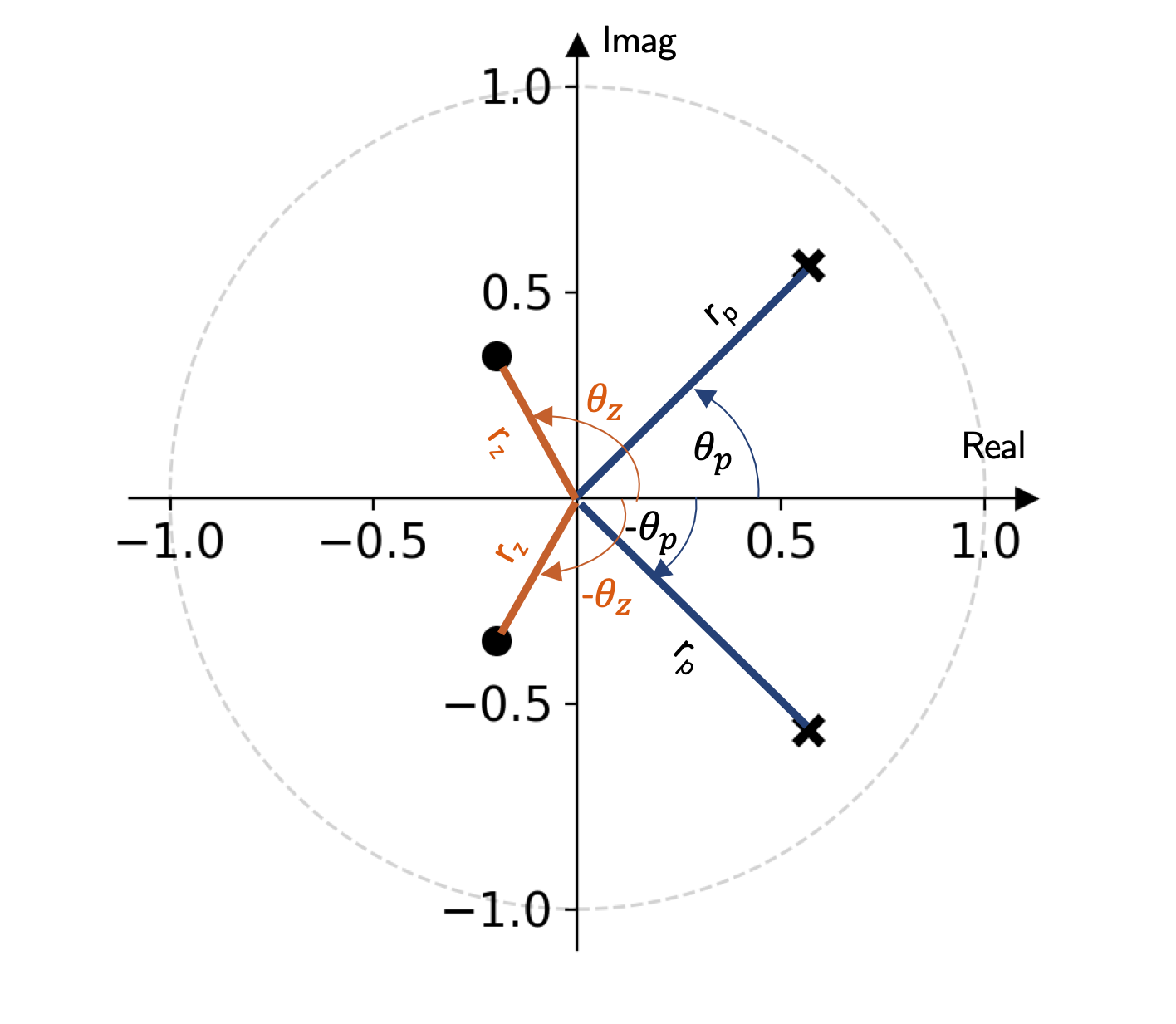
Fig. 1 - Magnitude and phase of poles and zeros.

Using these magnitude and phase expressions for the poles and zeros, and setting $g=1$, we can re-write the transfer function as follows:

\[ \begin{align} H(z) = \frac{(1-r_ze^{j\theta_z}z^{-1}) (1-r_ze^{-j\theta_z}z^{-1}) }{(1-r_pe^{j\theta_p}z^{-1}) (1-r_pe^{-j\theta_p}z^{-1})}\nonumber \end{align} \]

and if we expand the numerator and denominator, we obtain:

\[ \begin{align} H(z) &= \frac{1- (2r_z \cos\theta_z)z^{-1} + r_z^{2}z^{-2} }{1- (2r_p \cos\theta_p)z^{-1} + r_p^{2}z^{-2} }\nonumber \end{align} \]

which upon comparison to the transfer function of $H(z)$ in terms of its filter coefficients reveals the relationship between the magnitudes and phases of the poles and zeros and the filter coefficients (we can also observe here that the filter coefficients are real-valued due to the conjugate pairs of the poles and zeros):

\[\begin{split} \begin{align} b_0 &= 1 ; \hspace{0.2cm} b_1 = - 2r_z \cos\theta_z ; \hspace{0.2cm} b_2 = r_z^{2} \nonumber \\ a_1 &= - 2r_p \cos\theta_p ; \hspace{0.2cm} a_2 = r_p^{2} \nonumber \end{align} \end{split}\]

As opposed to individually specifying the filter coefficients $a_1, a_2, b_1, b_2$, we can rather design the digital filter by specifying the magnitudes and phases of the poles and zeros. For this biquad filter, we essentially have 4 parameters - $r_z, \theta_z, r_p, \theta_p$ from which we can obtain a wide range of filter types (low-pass, high-pass, bandpass, notch, etc.). In the interactive plot, you can modify these 4 parameters to see the relation between the positions of the poles and zeros and the magnitude/phase responses of the filters. Note that in the frequency domain plots, the x-axis is plotted in terms of a normalized frequency, $f/f_s$ for the range [0, 0.5] which corresponds to the range of $\omega T_s$ between [0, $\pi$].

# Setting up the plots
fig, axes = plt.subplot_mosaic([["top left", "top centre"],["top left", "bottom centre"]],figsize=(7.5,3))
plt.subplots_adjust(wspace=0.5,hspace=0.4)

# Create the unit circle
uc = patches.Circle((0,0), radius=1, fill=False, color='lightgray', ls='dashed')
axes["top left"].add_patch(uc)
 

# Plot the zeros and set marker properties    
t1, = axes["top left"].plot([], [], 'ko', ms=10)
plt.setp( t1, markersize=8.0, markeredgewidth=1.0,
          markeredgecolor='k', markerfacecolor='k')

# Plot the poles and set marker properties
t2, = axes["top left"].plot([], [], 'kx', ms=10)
plt.setp( t2, markersize=8.0, markeredgewidth=3.0,
          markeredgecolor='k', markerfacecolor='r')

axes["top left"].spines['left'].set_position('center')
axes["top left"].spines['bottom'].set_position('center')
axes["top left"].spines['right'].set_visible(False)
axes["top left"].spines['top'].set_visible(False)

axes["top left"].plot(1, 0, ">k", transform=axes["top left"].get_yaxis_transform(), clip_on=False)
axes["top left"].plot(0, 1, "^k", transform=axes["top left"].get_xaxis_transform(), clip_on=False)

# set the ticks
r = 1.1; 
axes["top left"].axis('scaled');
ticks_x = [-1, -0.5, 0.5, 1]; 
ticks_y = [-1, -0.5, 0.5, 1]; 
axes["top left"].set_xticks(ticks_x)
axes["top left"].set_yticks(ticks_y)
axes["top left"].text(1,0.1,'Real');
axes["top left"].text(0.1,1.1,'Imag');



lineMag, = axes["top centre"].plot([], [], 'k')
axes["top centre"].set_ylabel('Magnitude [dB]', color='k')
axes["top centre"].xaxis.set_major_formatter(FormatStrFormatter('%.1f'))
axes["top centre"].set_xlim([0, 0.5])
axes["top centre"].set_ylim([-50, 50])


# angles = np.unwrap(np.angle(h))
linePh, = axes["bottom centre"].plot([], [], 'k')
axes["bottom centre"].set_ylabel('Phase [radians]', color='k')
axes["bottom centre"].set_xlabel('Normalized Frequency (f/$f_s$)')
axes["bottom centre"].xaxis.set_major_formatter(FormatStrFormatter('%.1f'))
axes["bottom centre"].set_ylim([-np.pi, np.pi])
axes["bottom centre"].set_xlim([0, 0.5])
# axes["bottom centre"].axis('tight')

fs = 44100
Ts = 1/fs   # sampling period Ts
# Create the interactive plot
def update(rz = 0.8, rp = 0.95, thetaz=np.pi/4, thetap = np.pi/4):
    

    bo = 1;
    b1 = -2*np.cos(thetaz)*rp;
    b2 = rp**2;

    a1 = -2*np.cos(thetap)*rz;
    a2 = rz**2;

    b = [bo,b1,b2];
    a = [1,a1,a2];

    # FREQZ to get magnitude and phase
    w, h = signal.freqz(b,a)
    Mag = 20 * np.log10(abs(h))
    freq_axis = w/(2*np.pi)
    angles = np.unwrap(np.angle(h))
    
    # Get the poles and zeros
    p = np.roots(a)
    z = np.roots(b)


    lineMag.set_data(freq_axis, Mag)
    linePh.set_data(freq_axis, angles)
    t1.set_data(z.real, z.imag)
    t2.set_data(p.real, p.imag)
    fig.canvas.draw_idle()

print('Move the slider to see how the filter changes with the positions of the poles and zeros!')
interact(update, rz = (0,0.995,0.001), rp = (0,0.995,0.001), thetaz=(0,np.pi,np.pi/16), thetap=(0,np.pi,np.pi/16));
plt.show()
plt.tight_layout()

Move the slider to see how the filter changes with the positions of the poles and zeros!

Constrained Biquad filter#

A specific configuration of the biquad filter is to constrain it such that the poles and zeros lie on the same radial line, defined by angle $\theta_o$ in the complex plane, i.e. $\theta_{z} = \theta_{p} = \theta_o$. In this configuration, depending on the relative values of the magnitudes $r_z$ and $r_p$, the constrained biquad will behave as either a bandpass or a notch filter. The transfer function of the constrained biquad therefore simplifies to:

\[ \begin{align} H(z) &= \frac{(1-r_ze^{j\theta_o}z^{-1}) (1-r_ze^{-j\theta_o}z^{-1}) }{(1-r_pe^{j\theta_o}z^{-1}) (1-r_pe^{-j\theta_o}z^{-1})} = \frac{1- (2r_z \cos\theta_o)z^{-1} + r_z^{2}z^{-2} }{1- (2r_p \cos\theta_o)z^{-1} + r_p^{2}z^{-2} }\nonumber \end{align} \]

where there are only 3 parameters for designing the filter - $r_z, r_p, \theta_o$ and the filter coefficients are:

\[\begin{split} \begin{align} b_0 &= 1 ; \hspace{0.2cm} b_1 = - 2r_z \cos\theta_o ; \hspace{0.2cm} b_2 = r_z^{2} \nonumber \\ a_1 &= - 2r_p \cos\theta_o ; \hspace{0.2cm} a_2 = r_p^{2} \nonumber \end{align} \end{split}\]

The magnitude response of the constrained biquad is then given by

\[\begin{split} |H(e^{j\omega T_s})| = \frac{|(e^{j\omega T_s}- r_ze^{j\theta_o})| . |(e^{j\omega T_s}- r_ze^{-j\theta_o})|}{|(e^{j\omega T_s}- r_pe^{j\theta_o})| . |(e^{j\omega T_s}- r_pe^{j-\theta_o})|}\nonumber \\ \end{split}\]

where the minimum of the distances between $e^{j\omega T_s}$ and the zeros/poles occurs when $\omega T_s = \pm \theta_o$ (we can mathematically reason that out or we’ll look into the interactive plot below to see it). This then allows us to define a centre frequency where the resonance or notch will occur. Considering only the positive values of $\theta_o$ (i.e., for frequencies that will lie between 0 and $f_s/2$), we obtain the centre frequency, $f_c$ as:

\[\begin{split} \begin{align} \omega T_s &= \theta_o \nonumber \\ 2 \pi f_c T_s &= \theta_o \nonumber \\ f_c = \frac{\theta_o f_s}{2 \pi} \end{align} \end{split}\]

Hence the gain/attenuation at $f_c$$ becomes (substitute $\omega T_s = \theta_o$ into the magnitude expression):

\[\begin{split} |H(e^{j\omega T_s})| = \frac{|(1- r_z)| . |(1- r_ze^{-j(\theta_o + \omega T_s)})|}{|( 1 - r_p)| . |(1- r_pe^{-j(\theta_o + \omega T_s)})|}\nonumber \\ \end{split}\]

If $r_z > r_p$ or $r_p > r_z$, what type of filters do we obtain? You can either reason this out mathematically or look to the interactive plot below, where we observe how $r_z, r_p, and \theta_o$ affect the magnitude/phase response of the constrained biquad.

# Setting up the plots
fig, axes = plt.subplot_mosaic([["top left", "top centre"],["top left", "bottom centre"]],figsize=(7.5,3))
plt.subplots_adjust(wspace=0.5,hspace=0.4)

# Create the unit circle
uc = patches.Circle((0,0), radius=1, fill=False, color='lightgray', ls='dashed')
axes["top left"].add_patch(uc)
 

# Plot the zeros and set marker properties    
t1, = axes["top left"].plot([], [], 'ko', ms=10)
plt.setp( t1, markersize=8.0, markeredgewidth=1.0,
          markeredgecolor='k', markerfacecolor='k')

# Plot the poles and set marker properties
t2, = axes["top left"].plot([], [], 'kx', ms=10)
plt.setp( t2, markersize=8.0, markeredgewidth=3.0,
          markeredgecolor='k', markerfacecolor='r')

axes["top left"].spines['left'].set_position('center')
axes["top left"].spines['bottom'].set_position('center')
axes["top left"].spines['right'].set_visible(False)
axes["top left"].spines['top'].set_visible(False)

axes["top left"].plot(1, 0, ">k", transform=axes["top left"].get_yaxis_transform(), clip_on=False)
axes["top left"].plot(0, 1, "^k", transform=axes["top left"].get_xaxis_transform(), clip_on=False)

# set the ticks
r = 1.1; 
axes["top left"].axis('scaled');
ticks_x = [-1, -0.5, 0.5, 1]; 
ticks_y = [-1, -0.5, 0.5, 1]; 
axes["top left"].set_xticks(ticks_x)
axes["top left"].set_yticks(ticks_y)
axes["top left"].text(1,0.1,'Real');
axes["top left"].text(0.1,1.1,'Imag');



lineMag, = axes["top centre"].plot([], [], 'k')
axes["top centre"].set_ylabel('Magnitude [dB]', color='k')
axes["top centre"].xaxis.set_major_formatter(FormatStrFormatter('%.1f'))
axes["top centre"].set_xlim([0, 0.5])
axes["top centre"].set_ylim([-40, 40])


# angles = np.unwrap(np.angle(h))
linePh, = axes["bottom centre"].plot([], [], 'k')
axes["bottom centre"].set_ylabel('Angle [radians]', color='k')
axes["bottom centre"].set_xlabel('Normalized Frequency (f/$f_s$)')
axes["bottom centre"].xaxis.set_major_formatter(FormatStrFormatter('%.1f'))
axes["bottom centre"].set_ylim([-np.pi, np.pi])
axes["bottom centre"].set_xlim([0, 0.5])
# axes["bottom centre"].axis('tight')

# Create the interactive plot
def update(rz = 0.8, rp = 0.4, theta_o=np.pi/4):
    
    fig.canvas.draw_idle()
    
    b1 = -2*rz*np.cos(theta_o)
    b2 = rz**2
    a1 = -2*rp*np.cos(theta_o)
    a2 = rp**2
    bo = 1; ao = 1;

    b =[bo,b1,b2]
    a =[ao, a1, a2]
    

    # FREQZ to get magnitude and phase
    w, h = signal.freqz(b,a)
    Mag = 20 * np.log10(abs(h))
    freq_axis = w/(2*np.pi)
    angles = np.unwrap(np.angle(h))
    
    # Get the poles and zeros
    p = np.roots(a)
    z = np.roots(b)


    lineMag.set_data(freq_axis, Mag)
    linePh.set_data(freq_axis, angles)
    t1.set_data(z.real, z.imag)
    t2.set_data(p.real, p.imag)

print('Move the slider to see how the filter changes with the zero/pole magnitude and centre frequency!')
interact(update, rz = (0,0.99,0.01), rp = (0,0.99,0.01), theta_o=(0,np.pi,np.pi/16));
plt.show()
plt.tight_layout()

Move the slider to see how the filter changes with the zero/pole magnitude and centre frequency!

Filtering with Python#

So far, we’ve directly programmed equations for digital filter analysis to get a better understanding of what it is we’re actually doing. Python has many built-in functions that can also do this analysis for us, but it’s important that we always check the documentation to see exactly what it is these functions are doing. Many of the signal processing tools in Python can be found in the signal module within the scipy package. In the code below, we’ll highlight a few of these built-in functions and actually filter a signal and hear the result. We’ll make use of the following functions:

scipy.signal.freqz - Computes the frequency response of the filter
scipy.signal.tf2zpk - Computes the poles, zeros, and gain from the pole-zero factorisation form of a digital filter.
scipy.signal.lfilter - Filters an input signal with a filter whose b and a coefficients are specified.

In the code below, we’ll design a constrained biquad filter, configured as a bandpass filter to create a resonance boost at $4.5$ kHz.

# Read in the audio signal
x, fs = await read_wav_from_url(bass_sample) # read in the bass sample and get its sampling frequency
x=x*0.3 # reducing the level of the input so it does not clip after filtering.

# Design the constrained biquad filter to be a bandpass filter
# For this, we want that rp > rz.

fc = 4500 # centre frequency to boost (Hz)
thetao = (2*np.pi*fc)/fs # corresponding phase angle
rz = 0.1 # zero radius
rp = 0.95 # pole radius

# Specify filter coefficients
bo = 1; b1 = -2*np.cos(thetao)*rz; b2 = rz**2
a1 = -2*np.cos(thetao)*rp; a2 = rp**2
b =[bo,b1,b2] 
a =[1, a1, a2]

# Compute the frequency response of the filter using freqz:
f, H = signal.freqz(b,a, fs=fs) # freqz is a Python command to obtain freq. response of filter, H here is H(e^{j\omegaTs}), f is freq. in Hz. 
H_mag = 20*np.log10(np.abs(H))  # computer the magnitude
H_phase = np.angle(H) # compute phase

# Obtain poles and zeros
z, p, g = signal.tf2zpk(b, a) # This is a function to get  zeros, z, poles, p, and gain, g

# Filter the signal
x_filt = signal.lfilter(b, a, x) # This one line command is how we filter x with filter coefficients (b,a)!

# Audio to listen
print('Original Signal:')
IPython.display.display(Audio(x.T, rate=fs,normalize=False))
print('Filtered Signal:')
IPython.display.display(Audio(x_filt.T, rate=fs,normalize=False))

# Plotting
fig, ax = plt.subplot_mosaic([["top left", "top centre"],["top left", "bottom centre"]],figsize=(7.5,3))
plt.subplots_adjust(wspace=0.5,hspace=0.4)

# Make a Pole-zero plot
# generate a unit circle
phi = np.arange(0,2*np.pi + np.pi/16,np.pi/16)
unitc = np.exp(1j*phi)

ax["top left"].axvline(0, color='lightgrey')
ax["top left"].axhline(0, color='lightgrey')
ax["top left"].plot(z.real, z.imag, 'o',label = 'zeros')
ax["top left"].plot(p.real, p.imag, 'x', label = 'poles')
ax["top left"].plot(unitc.real, unitc.imag, '--', label='unit circle')
ax["top left"].set_xlabel('Real part of z')
ax["top left"].set_ylabel('Imaginary part of z')
ax["top left"].set_title('Pole-Zero Plot')
ax["top left"].set_xlim([-1.5,1.5])
ax["top left"].set_ylim([-1.5,1.5])
ax["top left"].set_aspect('equal', 'box')
# ax["top left"].legend(loc='upper right')

ax["top centre"].plot(f, H_mag)
ax["top centre"].set_xlabel('Frequency (Hz)')
ax["top centre"].set_ylabel('Magnitude (dB)')

ax["bottom centre"].plot(f, H_phase)
ax["bottom centre"].set_xlabel('Frequency (Hz)')
ax["bottom centre"].set_ylabel('Phase')
plt.tight_layout()
plt.show()



# Plot the original and filtered signals
fig,ax = plt.subplots(figsize=(7.5,3))
t = np.arange(0, len(x))/fs
ax.plot(t, x_filt, label='filtered signal')
ax.plot(t, x, label='original signal')
ax.set_xlabel('Time(s)')
ax.set_ylabel('Amplitude')
plt.tight_layout()
ax.legend()
plt.show()

Original Signal:

/var/folders/ng/90xk1wjn2014rw8nb9bql2200000gp/T/ipykernel_76841/3128879077.py:3: WavFileWarning: Chunk (non-data) not understood, skipping it.
  fs, x = wavfile.read('../audio/bass_sample.wav')

Filtered Signal:

Property	Z-transform
LINEARITY	\(\mathcal{Z}(ax[n] + by[n]) = aX(z) + bY(z)\) (where \(a\) and \(b\) are constants).
TIME-SHIFT	\(\mathcal{Z}(x[n-m]) = z^{-m}X(z)\)
CONVOLUTION	\(\mathcal{Z}(x[n] * y[n]) = X(z)Y(z)\)